generated from nmfs-opensci/NOAA-quarto-simple
-
Notifications
You must be signed in to change notification settings - Fork 32
/
Probability.qmd
532 lines (458 loc) · 23 KB
/
Probability.qmd
1
2
3
4
5
6
7
8
9
10
11
12
13
14
15
16
17
18
19
20
21
22
23
24
25
26
27
28
29
30
31
32
33
34
35
36
37
38
39
40
41
42
43
44
45
46
47
48
49
50
51
52
53
54
55
56
57
58
59
60
61
62
63
64
65
66
67
68
69
70
71
72
73
74
75
76
77
78
79
80
81
82
83
84
85
86
87
88
89
90
91
92
93
94
95
96
97
98
99
100
101
102
103
104
105
106
107
108
109
110
111
112
113
114
115
116
117
118
119
120
121
122
123
124
125
126
127
128
129
130
131
132
133
134
135
136
137
138
139
140
141
142
143
144
145
146
147
148
149
150
151
152
153
154
155
156
157
158
159
160
161
162
163
164
165
166
167
168
169
170
171
172
173
174
175
176
177
178
179
180
181
182
183
184
185
186
187
188
189
190
191
192
193
194
195
196
197
198
199
200
201
202
203
204
205
206
207
208
209
210
211
212
213
214
215
216
217
218
219
220
221
222
223
224
225
226
227
228
229
230
231
232
233
234
235
236
237
238
239
240
241
242
243
244
245
246
247
248
249
250
251
252
253
254
255
256
257
258
259
260
261
262
263
264
265
266
267
268
269
270
271
272
273
274
275
276
277
278
279
280
281
282
283
284
285
286
287
288
289
290
291
292
293
294
295
296
297
298
299
300
301
302
303
304
305
306
307
308
309
310
311
312
313
314
315
316
317
318
319
320
321
322
323
324
325
326
327
328
329
330
331
332
333
334
335
336
337
338
339
340
341
342
343
344
345
346
347
348
349
350
351
352
353
354
355
356
357
358
359
360
361
362
363
364
365
366
367
368
369
370
371
372
373
374
375
376
377
378
379
380
381
382
383
384
385
386
387
388
389
390
391
392
393
394
395
396
397
398
399
400
401
402
403
404
405
406
407
408
409
410
411
412
413
414
415
416
417
418
419
420
421
422
423
424
425
426
427
428
429
430
431
432
433
434
435
436
437
438
439
440
441
442
443
444
445
446
447
448
449
450
451
452
453
454
455
456
457
458
459
460
461
462
463
464
465
466
467
468
469
470
471
472
473
474
475
476
477
478
479
480
481
482
483
484
485
486
487
488
489
490
491
492
493
494
495
496
497
498
499
500
501
502
503
504
505
506
507
508
509
510
511
512
513
514
515
516
517
518
519
520
521
522
523
524
525
526
527
528
529
530
531
532
---
title: Probability
subtitle: The backbone of statistics!
bibliography: ../references.bib
---
<!-- COMMENT NOT SHOW IN ANY OUTPUT: Code chunk below sets overall defaults for .qmd file; these inlcude showing output by default and looking for files relative to .Rpoj file, not .qmd file, which makes putting filesin different folders easier -->
```{r setup, include=FALSE}
knitr::opts_chunk$set(echo = TRUE)
knitr::opts_knit$set(root.dir = rprojroot::find_rstudio_root_file())
source("../globals.R")
```
We've already address probability. When we stated the 95% confidence
interval means that if we make these intervals from 100 samples that we
expect 95 of them to contain the true mean, we are discussing
probability. An even easier example is flipping a coin. You probably
know there is a 50% chance of a coin landing on heads. That doesn't mean
given flip will be half heads and half tails. Both of these statements
refer to likely outcomes if we do something many, many times!
## What is probability?
To put it specifically, the probability of an outcome is its true
relative frequency, the proportion of times the event would occur if we
repeated the same process over and over again. We can describe the
probability if an outcome by considering all the potential outcomes and
how likely each is. If we describe all the outcomes, the total
probability must be equal to 1 (since frequency is typically measured as
a fraction!). Some probability distributions can be described
mathematically, others are a list of possible outcomes, and others are
almost impossible to solve. The "impossible" ones require simulations,
and we will return to this for our introduction to Bayesian analysis.
The simplest case is when we focus on outcomes for a single trait that
falls into specific categories. These outcomes are often *mutually
exclusive*, meaning only one can happen (like our heads and tails
example!), and lead to discrete probability distributions (meaning each
outcome has to be a specific value). Another example is rolling a
6-sided die. The die can only land on numbers 1 to 6 (so 2.57 is not an
option!).
```{r}
die_roll <- data.frame(Number = 1:6, Probability = rep(1/6,6))
die_roll$Number <- factor(die_roll$Number)
library(ggplot2)
ggplot(die_roll, aes(x=Number, y= Probability, fill=Number)) +
geom_col()
```
in this example, the probability of rolling a *6* is .167. You may see
this written as
$$
P[roll=6]= \frac{1}{6} \sim .167
$$Obviously when you roll a die you don't roll .167 of a 6. You roll a
1, 2, 3, 4, 5, or 6. Again, probability refers to the expected outcome
over multiple attempts.
Compare this to a continuous probability distribution, where the outcome
can take any value in a given range.
```{r}
ggplot(data = data.frame(x = c(-3, 3)), aes(x)) +
stat_function(fun = dnorm, n = 101, args = list(mean = 0, sd = 1), color = "orange")+
labs(y="Probability", x="Outcome")
```
Here's an odd outcome: Since the outcome can take on any value in a
given range, the chance of it being a *specific* value is 0. Think about
it this way - for any value you mention, I can zoom in more. For
example, if you ask the probability of **x** in the above graph being
equal to 0, we could zoom in to 0.0, or 0.00, or 0.000. At some limit of
resolution, the area under the curve (which denotes the probability and
would be found using integral calculus, which we won't do here) would be
equal to 0!
This may seem like an odd aside, but it is actually very important. It
explains why when we will discuss probabilities the probability of an
outcome being less than, more than, or between two values in upcoming
chapters. For example, we can note (again) that for a normal
distribution (what we see above and will (still eventually) define more
appropriately) that 67% of the data falls within one standard devation
for perfectly (very rare!) normally-distributed data.
```{r}
#function from https://dkmathstats.com/plotting-normal-distributions-in-r-using-ggplot2/
dnorm_one_sd <- function(x){
norm_one_sd <- dnorm(x)
# Have NA values outside interval x in [-1, 1]:
norm_one_sd[x <= -1 | x >= 1] <- NA
return(norm_one_sd)
}
ggplot(data = data.frame(x = c(-3, 3)), aes(x)) +
stat_function(fun = dnorm, n = 101, args = list(mean = 0, sd = 1), color = "orange")+
labs(y="Probability", x="Outcome") +
stat_function(fun = dnorm_one_sd, geom = "area", fill = "purple")
```
### What if more than one thing is of importance?
Sometimes we focus on the probability of more than one outcome for a
given event. This requires adding or combining probabilities. The first
step in doing this is deciding if the outcomes are *mutually exclusive*.
This means they can not occur in the same unit of focus. For example, we
could ask the probability of rolling a 1 or a 6, or of being \>2 and
\<-2. In both cases, a single outcome can't be both of these things, so
the outcomes are mutually exclusive. When this is the case, we simply
add the probabilities. This is sometimes called the *union* of two
outcomes.
Contrast this with when we want to know the probability of two things
occurring that may occur in the same unit. For example, assume our die
not only had dots on it, but these dots were a different color. For
example, odd numbers were blue and even numbers were red.
```{r}
colors <- c("blue" = "blue", "red" = "red")
die_roll$Color <- NA
die_roll[as.numeric(as.character(die_roll$Number)) %% 2 == 0, "Color"] <- "blue"
die_roll[as.numeric(as.character(die_roll$Number)) %% 2 != 0, "Color"] <- "red"
ggplot(die_roll, aes(x=Number, y= Probability, fill=Color)) +
geom_col() +
scale_fill_manual(values = colors)
```
Now, the probability of rolling any given group of numbers can be found
by adding probabilities since the outcomes are mutually exclusive. Same
for die color. However, what about the probability of rolling a blue
(even) outcome or a 6? Note we can't simply add these. Why not?
Because a single roll can result in a 6 and blue dots! So adding the
probability of getting blue dots (.5) and of getting a 6 (.167) will
double-count the 6. In other words, there is an an intersection of the
possible outcomes. So, the probability of rolling a 6 or blue is equal
to
$$
P[roll=blue] + P[roll=6] - P[roll=6 \ and \ blue]= \frac{1}{2} + \frac{1}{6} -\frac{1}{6}
$$
This is sometimes called the *general addition principle*.
If we are measuring multiple outcomes (note this slightly different than
the probability of two or more outcomes for a specific event), we need
to consider if the events are *independent*. This means the outcome of
one does not influence the outcome of the other. If this is true, the
probability of both events occurring can be found by simply multiplying
the probability of each (the *multiplication rule*). For example,
consider the probability of flipping a coin twice and seeing a heads
followed by a tails. We can write out all the options (T, HH, TH, TT);
assuming independence, the probability for each is $\frac{1}{4}$. We can
also say the probability of heads on the first flip is $\frac{1}{2}$ and
the probability of tails on the second flip is $\frac{1}{2}$;
multiplying these yields $\frac{1}{2}$.
Consider instead that we roll 2 dice and measure the sum of the rolls.
Since one roll does not influence the other, these are independent
events. As noted above, we can work out the probability distribution by
writing out all possible outcomes:
+------------+---+----------+----------+----------+----------+---------+---------+
| | | - \ | | | | | |
| | | \*Fi | | | | | |
| | | | | | | | |
| | | rst | | | | | |
| | | | | | | | |
| | | Dic | | | | | |
| | | | | | | | |
| | | e\ | | | | | |
| | | \*\* | | | | | |
+------------+---+----------+----------+----------+----------+---------+---------+
| | | 1 | 2 | 3 | 4 | 5 | 6 |
+------------+---+----------+----------+----------+----------+---------+---------+
| - \* Sec | 1 | ( 1 ,1) | ( 1 ,2) | ( 1 ,3) | - \ | ( 1 ,5) | ( 1 ,6) |
| | | | | | \*(1 | | |
| ond | | | | | | | |
| | | | | | , | | |
| Dic | | | | | | | |
| | | | | | 4 | | |
| e\ | | | | | | | |
| \*\* | | | | | )\ | | |
| | | | | | \*\* | | |
+------------+---+----------+----------+----------+----------+---------+---------+
| | 2 | ( 2 ,1) | ( 2 ,2) | - \ | ( 2 ,4) | ( 2 ,5) | ( 2 ,6) |
| | | | | \*(2 | | | |
| | | | | | | | |
| | | | | , | | | |
| | | | | | | | |
| | | | | 3 | | | |
| | | | | | | | |
| | | | | )\ | | | |
| | | | | \*\* | | | |
+------------+---+----------+----------+----------+----------+---------+---------+
| | 3 | ( 3 ,1) | - \ | ( 3 ,3) | ( 3 ,4) | ( 3 ,5) | ( 3 ,6) |
| | | | \*(3 | | | | |
| | | | | | | | |
| | | | , | | | | |
| | | | | | | | |
| | | | 2 | | | | |
| | | | | | | | |
| | | | )\ | | | | |
| | | | \*\* | | | | |
+------------+---+----------+----------+----------+----------+---------+---------+
| | 4 | - \ | ( 4 ,2) | ( 4 ,3) | ( 4 ,4) | ( 4 ,5) | ( 4 ,6) |
| | | \*(4 | | | | | |
| | | | | | | | |
| | | , | | | | | |
| | | | | | | | |
| | | 1 | | | | | |
| | | | | | | | |
| | | )\ | | | | | |
| | | \*\* | | | | | |
+------------+---+----------+----------+----------+----------+---------+---------+
| | 5 | ( 5 ,1) | ( 5 ,2) | ( 5 ,3) | ( 5 ,4) | ( 5 ,5) | ( 5 ,6) |
+------------+---+----------+----------+----------+----------+---------+---------+
| | 6 | ( 6 ,1) | ( 6 ,2) | ( 6 ,3) | ( 6 ,4) | ( 6 ,5) | ( 6 ,6) |
+------------+---+----------+----------+----------+----------+---------+---------+
Now assume we want to know the probability of the sum of the dice being
equal to 5. If we assume independence, the the probability of rolling a
sum of 5 (highlighted cells above) is $\frac{4}{36}$.
We could also simulate the outcome
```{r}
library(reshape2)
number_of_rolls <- 100000
sum_of_rolls <- data.frame(index = 1:number_of_rolls, Sum = NA)
for (i in 1:number_of_rolls){
dice_roll_trial <- sample(1:6, size = 2, replace = TRUE)
sum_of_rolls$Sum[i] <- sum(dice_roll_trial)
}
sum_of_rolls_df <- dcast(sum_of_rolls, Sum ~ "Probability", length )
sum_of_rolls_df$Probability <- sum_of_rolls_df$Probability/number_of_rolls
ggplot(sum_of_rolls_df, aes(x=Sum, y=Probability)) +
geom_col(fill="orange", color="black") +
labs(y="Probability")+
scale_x_continuous(breaks = c(2:12))
```
Notice here we find the probability of rolling a sum of 5 is
`r sum_of_rolls_df[sum_of_rolls_df$Sum == 5, "Probability"]` which is
very close to $\frac{4}{36}$.
To find the probability using math, we have to note that the dice rolls
are independent. For example, even though we only want a **4** on the
second dice if we roll a **1** on the first dice, the roll of the first
die does not influence the roll of the second. We should also note the
desired outcomes are mutually exclusive. So we can find the probability
of each happening and then add them. It's easy to see how probability
can get complicated!
## Conditional Probability
Unlike our coin example, sometimes a first event occurring does
influence the probability of a second event.
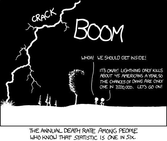{fig-alt="Two stick figures are walking outside. Lightning strikes. One mentions they should go inside. The other notes only 45 Americans are killed by a lightning strike each year, so the chances of dying are less than one in 7,000,000"}
In a similar vein, although the risk of shark attack is low, it
increases dramatically if you swim in the ocean.
Unlike our previous examples, we now have 2 events (lets call them A and
B), and the probability of both occurring is equal to
$$
P[A \ and \ B] = P[A] \ P[B|A]
$$
which can be read as "the probability of A and B occurring is equal to
the probability of A multiplied by the probability of B given A occurs".
Note if A and B are independent, this reduces to the multiplication
rule.
We can extend this by noting
$$
P[A \ and \ B] = P[A] \ P[B|A] \\
P[A \ and \ B] = P[B] \ P[A|B] \\
P[A] \ P[B|A] = P[B] \ P[A|B] \\
P[A|B] = \frac{P[B|A]*P[A]}{P[B]}
$$
This rule is known as *Bayes' Theorem*. We will return to this when we
discuss *Bayesian* analysis, but we can use it here for demonstration.
For our lightning example, we could use some (pretend) numbers to
understand the risk and Bayes' Theorem. First, let A be the probability
of being outside in a lightning storm. B is then the probability of
getting struck by lightning, , and P\[B\|A\] is the probabiity of
getting struck by lightning given that you are outside in a lightning
storm (hint: it's much higher than the P\[B\]).
Here's anoher similar (in concept) example. Medical trials are designed
to test the effectiveness of drugs or treatments. In these trials, drug
efficacy is considered by comparing outcomes in people who receive the
drug or treatment compared to those who receive a placebo (such as a
sugar pill). Note this only works if participants do not know which
group (drug vs placebo) they are in (why?). In a given trial, people who
receive the drug recover 60% of the time (or avoid some other adverse
outcome). This may seem good, but it's only relevant when compared to
the placebo group. What if people receiving the placebo recovered 80% of
the time? Also, if we know the probability of recovering without the
drug, we can consider the total probability of recovery. For now, let's
assume that 20% of people who receive the placebo recover.
We could use a tree diagram to consider possible options:
```{r}
library(DiagrammeR)
bayes_probability_tree <- function(prior, true_positive, true_negative, label1 = "Prior",
label2 = "Complimentary Prior", label3 = "True Positive",
label4 = "False Negative", label5 = "False Positive",
label6 = "True Negative") {
if (!all(c(prior, true_positive, true_negative) > 0) && !all(c(prior, true_positive, true_negative) < 1)) {
stop("probabilities must be greater than 0 and less than 1.",
call. = FALSE)
}
c_prior <- 1 - prior
c_tp <- 1 - true_positive
c_tn <- 1 - true_negative
round4 <- purrr::partial(round, digits = 5)
b1 <- round4(prior * true_positive)
b2 <- round4(prior * c_tp)
b3 <- round4(c_prior * c_tn)
b4 <- round4(c_prior * true_negative)
bp <- round4(b1/(b1 + b3))
labs <- c("X", prior, c_prior, true_positive, c_tp, true_negative, c_tn, b1, b2, b4, b3)
tree <-
create_graph() %>%
add_n_nodes(
n = 11,
type = "path",
label = labs,
node_aes = node_aes(
shape = "circle",
height = 1,
width = 1,
x = c(0, 3, 3, 6, 6, 6, 6, 8, 8, 8, 8),
y = c(0, 2, -2, 3, 1, -3, -1, 3, 1, -3, -1))) %>%
add_edge(
from = 1,
to = 2,
edge_aes = edge_aes(
label = label1
)
) %>%
add_edge(
from = 1,
to = 3,
edge_aes = edge_aes(
label = label2
)
) %>%
add_edge(
from = 2,
to = 4,
edge_aes = edge_aes(
label = label3
)
) %>%
add_edge(
from = 2,
to = 5,
edge_aes = edge_aes(
label = label4
)
) %>%
add_edge(
from = 3,
to = 7,
edge_aes = edge_aes(
label = label5
)
) %>%
add_edge(
from = 3,
to = 6,
edge_aes = edge_aes(
label = label6
)
) %>%
add_edge(
from = 4,
to = 8,
edge_aes = edge_aes(
label = "="
)
) %>%
add_edge(
from = 5,
to = 9,
edge_aes = edge_aes(
label = "="
)
) %>%
add_edge(
from = 7,
to = 11,
edge_aes = edge_aes(
label = "="
)
) %>%
add_edge(
from = 6,
to = 10,
edge_aes = edge_aes(
label = "="
)
)
message(glue::glue("The probability of having {label1} after testing {label3} is {bp}"))
print(render_graph(tree))
invisible(tree)
}
#first example
bayes_probability_tree(prior = 0.5, true_positive = 0.8, true_negative = 0.8, label1 = "medicine", label2 = "placebo",
label3 = "cured", label4 = "not cured",
label5 = "cured", label6 = "not cured")
```
This tree let's us consider multiple things. We can see the probability
of being cured is .5, but 80% of those come from the group receiving
medicine (again, the P\[being cured\|given medicine\]). WE could also
derive this using Bayes Theorem.
\$\$ P\[being cured\|medicine\] =
\frac{P[receiving \ medicine|cured]P[being \ cured]}{P[receiving \ medicine]}
\\ P\[being cured\|medicine\] = \frac{.8 * .5}{.5} \\ P\[being
cured\|medicine\] = .8
\$\$
One more example. Instead of medical trials, let's focus on medical
screenings. These are used to identify patients who have a condition,
but there are no perfect tests. A test may give a *false positive*,
meaning it says a condition exists when it does not. A test can also
give a *false negative*, meaning it finds a condition does not exist
when it really does. Both of these present issues for patients and
explain why series of tests are often used before more invasive
procedures are employed.
For example, assume a procedure is used to assess skin cancer. This
cancer occurs at a frequency of .00021 in the general population. The
test is fairly accurate; if a patient has cancer, the screening will
correctly identify if 95% of the time. However, the probability of a
false positive is .01. Given these numbers, how worried should a person
be about a positive test?
Although the test seems to be good, note the prevalence of a false
positive is far higher than the prevalence of cancer! This means most
positives will likely be false. To quantify this, let A be the
probability of cancer and B be the probability of a positive screening.
So,
$$
P[A|B] = \frac{.95 \ * .00021}{.95 \ * \ .0021+.01*.9779} \\
P[A|B] = .169
$$
In other words, only 17% of people with positive screenings actually
have cancer.
To show this in a probability tree:
```{r}
bayes_probability_tree(prior = 0.0021, true_positive = 0.95, true_negative = 0.99, label1 = "cancer",
label2 = "not cancer",
label3 = "positive",
label4 = "negative",
label5 = "positive",
label6 = "negative")
```
## Related Ideas
False results are integral to the ideas of test *specificity* and
*sensitivity* @lalkhen2008. A specific test will yield few false
negatives, while a sensitive test will yield few false positives. Put
another way (from Lalken & McCluskey (2008): "A test with 100%
sensitivity correctly identifies all patients with the disease", and " a
test with 100% specificity correctly identifies all patients without the
disease". True and false results also impact predictive values.
+------------------+----------------------------------+--------------------+
| | **Condition** | |
+------------------+----------------------------------+--------------------+
| **\ | Present | Absent |
| \ | | |
| ** | | |
| | | |
| **Test Outcome** | | |
+------------------+----------------------------------+--------------------+
| Positive | True Positive | False positive |
+------------------+----------------------------------+--------------------+
| Negative | False negative | True Negative |
+------------------+----------------------------------+--------------------+
| | Sensitivity= | Specificity = |
| | | |
| | True Positive/ Condition present | True negative/ |
| | | |
| | | Condition negative |
+------------------+----------------------------------+--------------------+
These ideas can also be related to power. We will return to this
visualization in future chapters.

## Next steps
Now that we've discussed probability, we can move into the wild world of
p-values and discuss how they relate to estimation!