When using facet_grid(), plot lines do not extend all the way to the y-axis #254
Comments
|
Please, follow the procedure described at: #205 In your case, the code looks like this: library(survival)
library(survminer)
fit <- survfit(Surv(survival, censor) ~ geneA + geneB , data = ss)
ggsurvplot(fit, legend = 'none', facet.by = "Sex") |
|
Thanks for your feedback,
I tried out 'facet.by' but this did not appear to fix the issue. It still
results in drawing line segments that do not reach the y-axis. This time
however, changing the order of the factor levels did not result in the
lines being drawn correctly, like facet_grid() seemed to do in my original
post.
I'm attaching two plots, one where I did not use any facets and the other
which uses 'facet.by = gender'. This is a reduced dataset compared to my
original one as I was trying to simplify things to narrow down where the
problem originated. I'll include a printout of the survfit below:
Call: survfit(formula = Surv(survival, censor) ~ gender + genotype, data =
ss2)
n events median 0.95LCL 0.95UCL
gender=Female, genotype=+/+/- 21 13 134 113 NA
gender=Female, genotype=+/+/+ 8 3 NA 124 NA
gender=Male, genotype=+/+/- 24 8 NA 407 NA
gender=Male, genotype=+/+/+ 8 1 NA NA NA
Code:
fit <- survfit(Surv(survival, censor) ~ gender + genotype, data = ss2)
First plot:
ggsurvplot(fit)
Second plot:
ggsurvplot(fit, facet.by="gender")
Thanks very much for your input.
Chris
…On Wed, Oct 4, 2017 at 1:49 PM, Alboukadel KASSAMBARA < ***@***.***> wrote:
Please, follow the procedure described at: #205
<#205>
In your case, the code looks like this:
library(survival)
library(survminer)

fit <- survfit(Surv(survival, censor) ~ geneA + geneB , data = ss)
ggsurvplot(fit, legend = 'none', facet.by = "Sex")
—
You are receiving this because you authored the thread.
Reply to this email directly, view it on GitHub
<#254 (comment)>,
or mute the thread
<https://github.com/notifications/unsubscribe-auth/Ae_A-1umY4aGZ2g00qCxIkxAzZ1jZ7uXks5so9NRgaJpZM4Psab2>
.
|
|
Please provide a reproducible example with a sample of your data. To include data in a question, use dput() to generate the R code to recreate it. For example, to recreate the mtcars dataset in R, I’d perform the following steps:
|
|
The demo data set is not attached to your message... |
|
Feel free to send the demo data set or to incorporate it in the script itself. The only important thing is to make sure that your script can be executed, so that we can easily reproduce the issue in order to fix it. Thank you in advance |
|
Hi, Note that, When lefting github comment via e-mail reply, attached files don't follow the message. You can send me directly the files at: alboukadel.kassambara@gmail.com Thanks |
|
My mistake, didn't realize that was happening. My example dataset and code: My output plot:
|

|
I can see know where is the problem. I'll work on it. The output should look like this: library(survminer)
library(survival)
library(magrittr)
surv_fit(Surv(survival, censor) ~ genotype,
         data = df, group.by = "gender") %>%
  ggsurvplot(ggtheme = theme_bw()) %>%
  purrr::map(function(ggsurv) {ggsurv$plot}) %>%
  ggpubr::ggarrange(plotlist = .)
|

|
I am having the same issue. The code you posted above fixes the truncated segments on the plots, but I couldn't use all the graphical parameters I'm typically using when using Things like Is there any other fix for this issue? |
|
same issue...any update on solution? |
|
@kassambara, when using instead of to circumvent the plotting issue, and chosing to display the p-value with Also, how can I access the statistics details of the test(s), in addition to the p-value(s)? I need to finalize an analysis this week and adding my plot in the document reminded me that it is still unclear to me what is done under the hood for this figure. |
|
I'm having the same problem with the survplot_facet function, The survival curve displayed correctly when I plotted the survival curve using the normal ggsurvplot function. However, the parts of the plot line disappeared when I tried to facet the graph similar to what happened above. The modification of the code to use group.by circumvent the issue but the graph did not come out as I wanted. I am suspecting that there is something wrong with the facet function but cannot figure out the way to correct it. Could you please check if there there is something wrong with my code? Below is the dataset and the code I used. Iso <- structure(list(Sample = 1:70, Treatment = structure(c(1L, 1L, fit <- survfit(Surv(Time, Event) ~Dose+Treatment , data = Iso) ggsurv$plot + theme_bw()+facet_grid(Treatment~Dose) Thank you very much in advance for your help. |


|
@kassambara When faceting, I either get the error:
The workaround you describe above does not allow for multiple factors in the Surv function. For example Any updates or workarounds appreciated! |
|
I believe I've found the bug that prevents the faceting from properly drawing the lines when there are more than one strata. I've attached the image of the data.frame created by ggsurvplot. See how the strata column is correctly built (red arrow), but the factors are all equal to the first level of strata combination (blue arrow).
I've worked around it by manually adding the initial states of all factor combinations and plot with the usual ggplot2's geom_step: The plot produced is below (labels in portuguese, sorry!):
I still have to learn how to add the crosses for the censoring, but that shouldn't be very hard. |


|
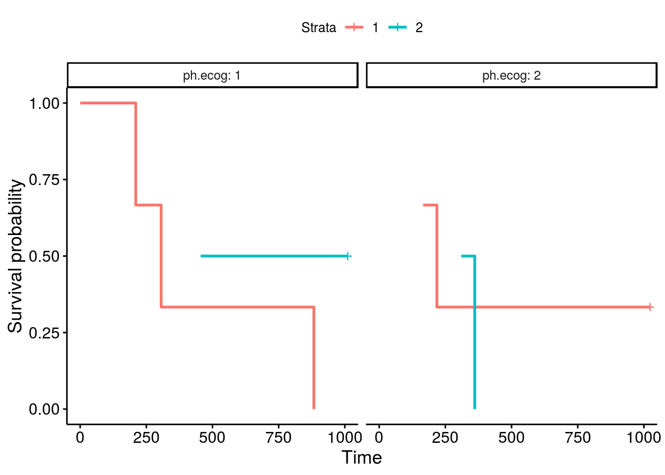
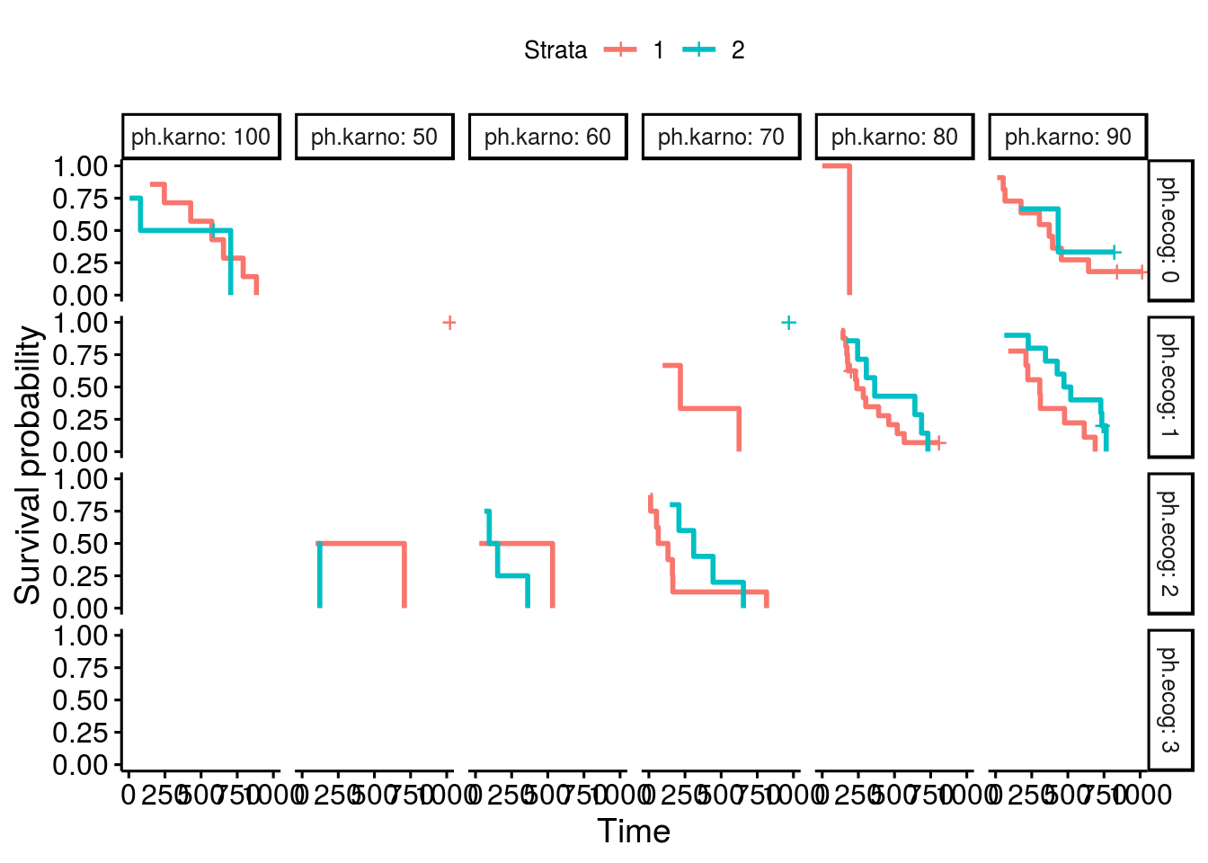
I have also notice the same issue, miss labled stratas, as in the thread from "bernardose" on Nov 13, 2018. Below is my proposed fix: Test case 1which is actural the first 10 data points in lung: Plot with issuesOne can facet the sex=1 and sex=2 plots by ph.ecog values:
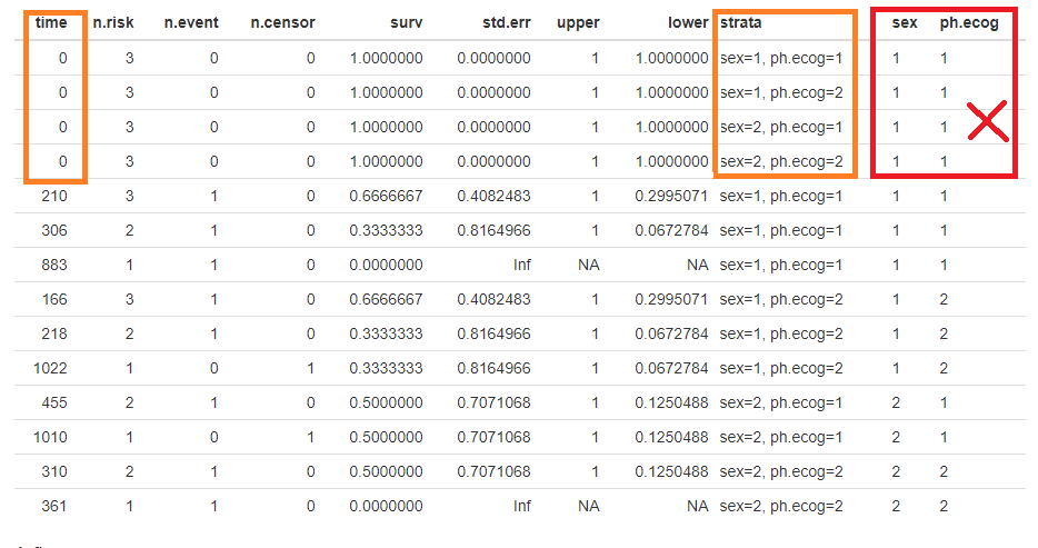
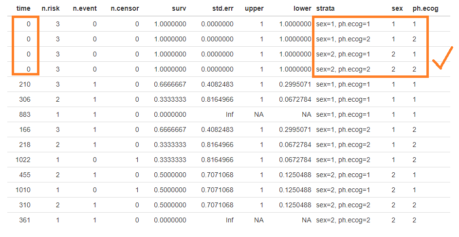
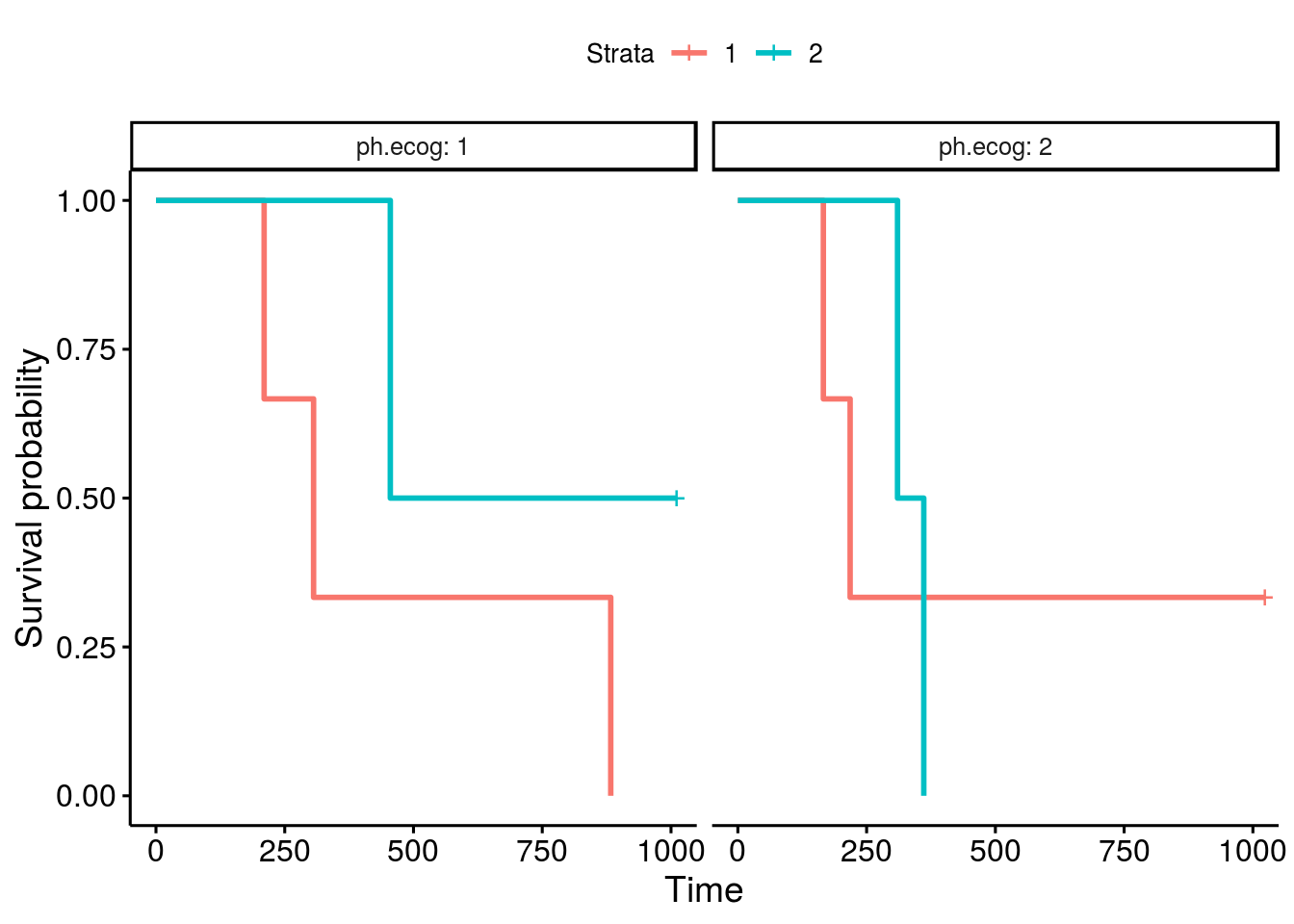
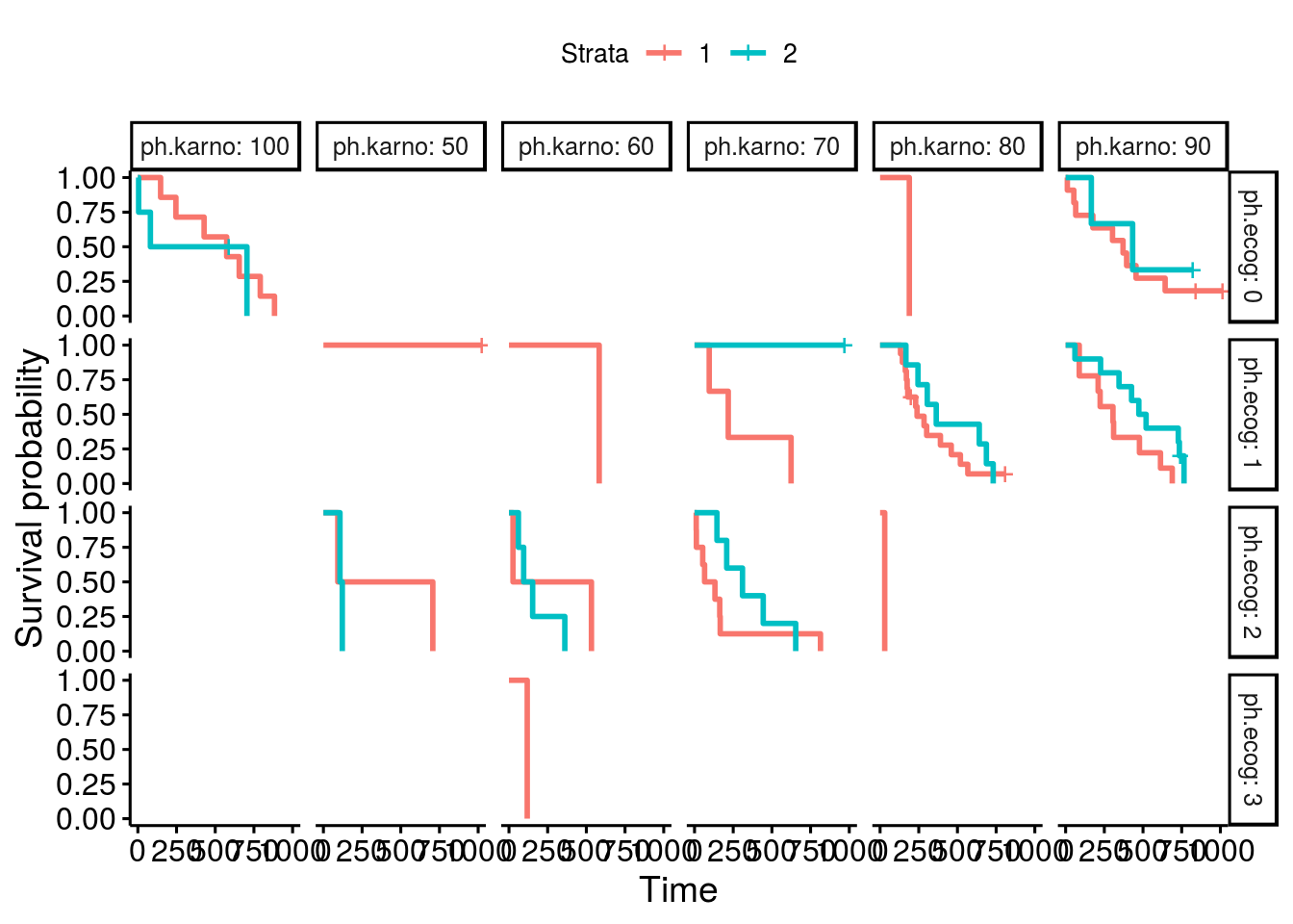
Here comes the problem. The function ggsurvplot_facet() missed the first intervals for each survival plot. It was caused by the returning dataframe .$data, where the starting point was not set correctly, shown in the table below. Pay attention to the first 4 rows and the last 2 columns, sex and ph.ecog values are not set correctly, compare to the column strata values. A fixThe function, that causes the problem of missing the first interval in a survival plot, was function .connect2origin(), which was called by ggsurvplot_df(), which was called by ggsurvplot_core(), which was called by ggsurvplot_facet(). The orginial span .connect2origin() is as follows: The code basically created and copy the origin for each subplot/faceted plot from the very first one. I have added a block of code to modify the origin per strata per facet as follows as .connect2origin_fix(): Now the fixed table is as: Test case 2This case is with more choices of strata and facets. Note that there is no data points for certain strata and facet.
Download and use the fixCheck the README.md file: |
|
To fix this issue, we can rewrite the .connect2origin <- function(d, ...){
n.risk <- strata <- NULL
if("n.risk" %in% colnames(d)){d <- dplyr::arrange(d, dplyr::desc(n.risk))}
origin <- d %>% distinct(strata, .keep_all = TRUE)
origin[intersect(c('time', 'n.censor', 'std.err', "n.event"), colnames(origin))] <- 0
origin[c('surv', 'upper', 'lower')] <- 1.0
dplyr::bind_rows(origin, d)
} |
|
Fixed now, thanks! Install the latest developmental version and test this: df <- structure(list(ID = c("897", "838", "839", "847", "842", "801",
"718", "726", "730", "925", "926", "931", "936", "952", "953",
"884", "891", "894", "895", "899", "902", "905", "908", "914",
"807", "841", "844", "837", "846", "815", "818", "819", "822",
"800", "722", "728", "809", "892", "900", "724", "885", "939",
"940", "946", "810", "943", "934", "840", "947", "727", "937",
"955", "954", "948", "889", "935", "929", "798", "716", "816",
"824"), gender = structure(c(2L, 1L, 1L, 2L, 2L, 1L, 2L, 2L,
2L, 1L, 1L, 2L, 2L, 2L, 2L, 1L, 2L, 2L, 2L, 1L, 2L, 2L, 1L, 2L,
1L, 1L, 2L, 1L, 2L, 1L, 2L, 2L, 2L, 1L, 2L, 2L, 1L, 1L, 1L, 1L,
1L, 2L, 1L, 1L, 1L, 1L, 1L, 1L, 1L, 2L, 2L, 2L, 2L, 1L, 2L, 2L,
2L, 1L, 1L, 1L, 2L), .Label = c("Female", "Male"), class = "factor"),
genotype = structure(c(1L, 1L, 1L, 1L, 1L, 1L, 1L, 1L, 1L,
1L, 1L, 1L, 1L, 1L, 1L, 1L, 1L, 1L, 1L, 1L, 1L, 1L, 1L, 1L,
2L, 2L, 2L, 2L, 2L, 2L, 2L, 2L, 2L, 2L, 2L, 2L, 1L, 1L, 1L,
1L, 1L, 1L, 1L, 1L, 1L, 1L, 1L, 1L, 1L, 1L, 1L, 1L, 1L, 1L,
1L, 1L, 1L, 2L, 2L, 2L, 2L), .Label = c("+/+/-", "+/+/+"), class = "factor"),
survival = c(122L, 394L, 394L, 394L, 394L, 400L, 401L, 401L,
401L, 519L, 519L, 519L, 519L, 519L, 519L, 520L, 520L, 520L,
520L, 520L, 520L, 520L, 520L, 520L, 72L, 394L, 394L, 394L,
394L, 399L, 399L, 399L, 399L, 400L, 401L, 401L, 75L, 78L,
80L, 83L, 87L, 106L, 106L, 113L, 123L, 125L, 126L, 134L,
143L, 151L, 164L, 171L, 203L, 226L, 239L, 379L, 407L, 88L,
124L, 159L, 299L), censor = c(0L, 0L, 0L, 0L, 0L, 0L, 0L,
0L, 0L, 0L, 0L, 0L, 0L, 0L, 0L, 0L, 0L, 0L, 0L, 0L, 0L, 0L,
0L, 0L, 0L, 0L, 0L, 0L, 0L, 0L, 0L, 0L, 0L, 0L, 0L, 0L, 1L,
1L, 1L, 1L, 1L, 1L, 1L, 1L, 1L, 1L, 1L, 1L, 1L, 1L, 1L, 1L,
1L, 1L, 1L, 1L, 1L, 1L, 1L, 1L, 1L)), row.names = c(NA, -61L
), class = "data.frame", .Names = c("ID", "gender", "genotype",
"survival", "censor"))
library(survival)
library(survminer)
fit <- survfit(Surv(survival, censor) ~ gender + genotype, data = df)
ggsurvplot(fit, facet.by="gender")Should give this output:
|

…and so facet. fix for kassambara#254, kassambara#363
Expected behavior
Survival plot lines will appear to extend all the way to the y-axis on both facets of a plot.
Actual behavior
When using ggsurvplot() with facet_grid() on a survfit object, the second level of the faceting factor has line-segments displayed rather than extending the lines all the way to the y-axis. The first faceting factor does not appear to have this problem. When the factor levels are reversed, the new second level now displays line segments rather than extending to the y-axis.
In my example the survival fit is created with two genotypes and sex as factors. I am faceting the plots by sex, F for female and M for male. First the male curve has truncated line segments, but when the factor levels are reversed the male lines are drawn correctly but the female lines now don't extend to the y-axis.
I suspect that without faceting, the overlapping lines that converge at the y-axis are being masked in a particular order. When facet_grid() is used the masking is still taking place but now it becomes revealed. Is there a way to correct this? I've been unable to find any references to this issue elsewhere, and no features to control how the lines get drawn or if line masking can be enabled/disabled in the ggsurvplot package.
Steps to reproduce the problem
library(survival)
library(ggplot2)
library(survminer)
library(dplyr)
fit <- survfit(Surv(survival, censor) ~ geneA + geneB + Sex, data = ss)
ggsurvplot(fit, legend = 'none') +
facet_grid(.~Sex)
#default factor levels, F then M
#reverse the factor levels, M then F
ss$Sex <- factor(ss$Sex, levels=c('M','F'))
session_info()R version 3.4.0 (2017-04-21)
Platform: x86_64-w64-mingw32/x64 (64-bit)
Running under: Windows 7 x64 (build 7601) Service Pack 1
Matrix products: default
locale:
[1] LC_COLLATE=English_United States.1252 LC_CTYPE=English_United States.1252
[3] LC_MONETARY=English_United States.1252 LC_NUMERIC=C
[5] LC_TIME=English_United States.1252
attached base packages:
[1] stats graphics grDevices utils datasets methods base
loaded via a namespace (and not attached):
[1] compiler_3.4.0 tools_3.4.0
The text was updated successfully, but these errors were encountered: