CoastSat's shoreline mapping alogorithm uses an image classification scheme to label each pixel into 4 classes: sand, water, white-water and other land features. While this classifier has been trained using a wide range of different beaches, it may be that it does not perform very well at specific sites that it has never seen before.
For this reason, we provide the possibility to re-train the classifier by adding labelled data from new sites. This can be done very quickly and easily by using this Jupyter Notebook.
Let's take this example, Playa Chañaral in the Atacama desert, Chile. At this beach, the sand is extremely white and the default classifier is not able to label correctly the sand pixels:
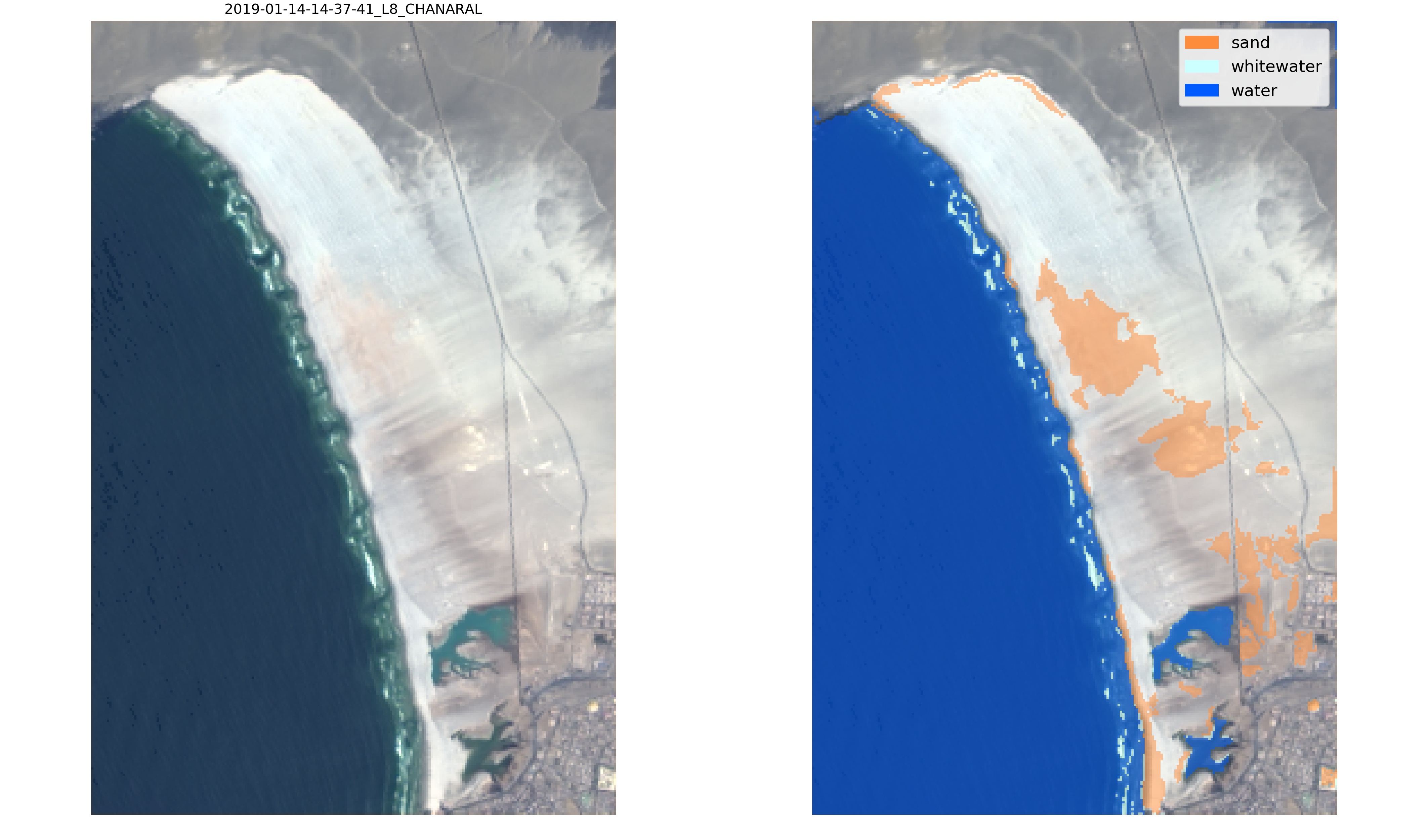
To overcome this issue, we can generate training data for this site by labelling new images.
Download the new images to be labelled and then call the function SDS_classify.label_images(metadata,settings), an interactive tool will pop up for quick and efficient labelling:
You only need to label sand pixels, as water and white-water looks the same everywhere in the world. You can label 2-3 images in a few minutes with the interactive tool and then the new labels can be used to re-train the classifier. The labelling tool uses flood fill to speed up the selection of sand pixels and you can tune the tolerance of the flood fill function in settings['tolerance'].
You can then train a classifier with the newly labelled data. Different classification schemes exist, in this example we use a Multilayer Perceptron (Neural Network) with 2 layers, one of 100 neurons and one of 50 neurons. The training data is first divided in train and split, so that we can evaluate the accuracy of the classifier and plot a confusion matrix.
X_train, X_test, y_train, y_test = train_test_split(X, y, test_size=0.3, shuffle=True, random_state=0)
classifier = MLPClassifier(hidden_layer_sizes=(100,50), solver='adam')
classifier.fit(X_train,y_train)
print('Accuracy: %0.4f' % classifier.score(X_test,y_test))
y_pred = classifier.predict(X_test)
label_names = ['other land features','sand','white-water','water']
SDS_classify.plot_confusion_matrix(y_test, y_pred,classes=label_names,normalize=False);

Finally, the new classifier can be applied to the satellite images, for visual inspection by calling the function SDS_classify.evaluate_classifier(classifier,metadata,settings) which will save the classified images in /evaluation:
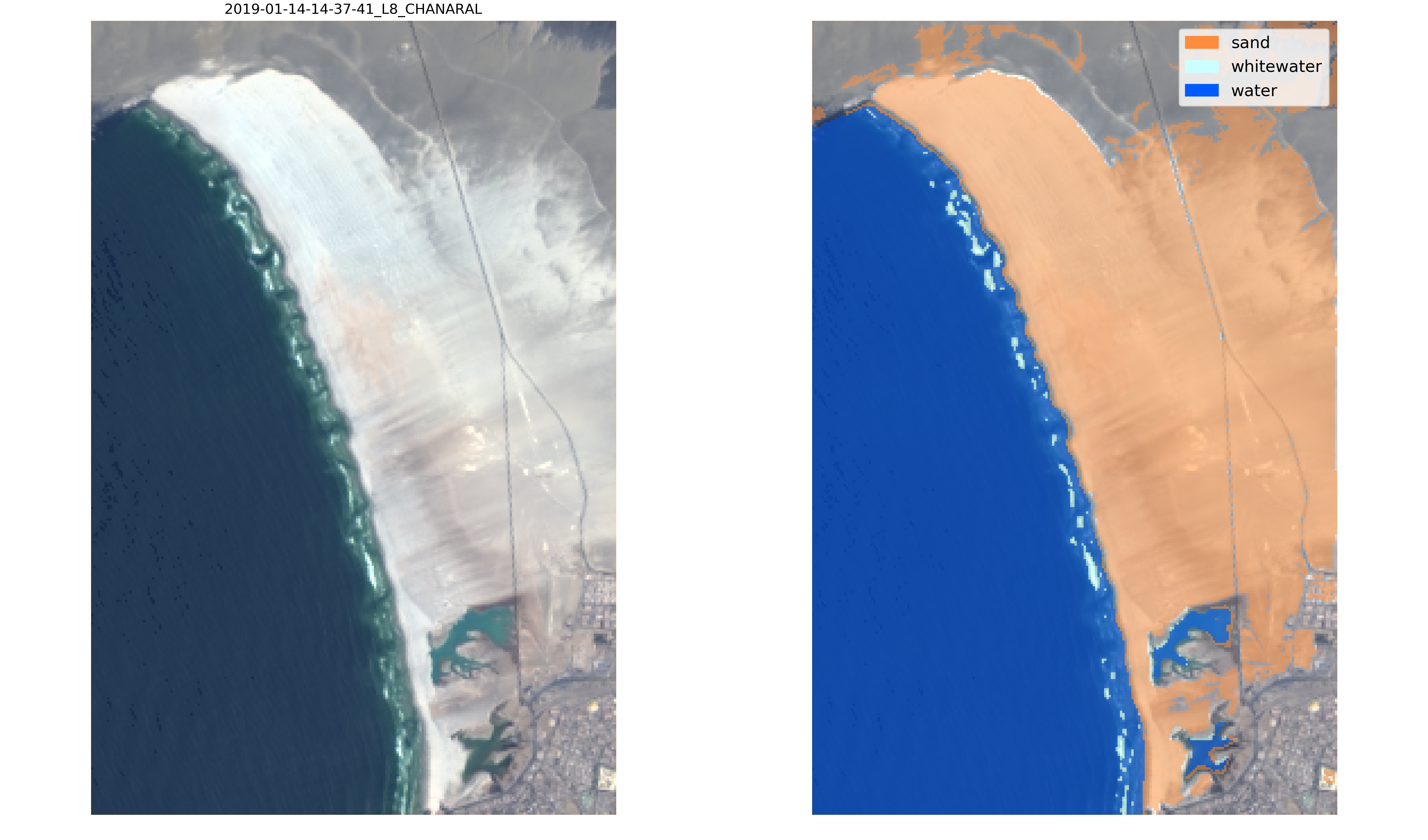
Now, this new classifier labels correctly the sandy pixels of the Atacama desert and will provide more accurate satellite-derived shorelines at this beach!