ANOVA - Analysis of Variance

Today, we will be learning ANOVA, a generalized form of comparing mean across multiple groups. Agenda today:

1. Compare t-tests and ANOVA
2. Differentiate between variance between groups and variance within groups
3. Learn to calculate ANOVA
4. Implement ANOVA in Python
   • using statsmodels

1. T tests or ANOVA?

ANOVA or Analysis Of Variance provides a statistical test of whether two or more population means are equal, and therefore generalizes the t-test beyond two means.

Suppose we want to compare whether multiple groups differ in some type of measures. For example, we have collected mood data grouped by four types of weather - sunny, raining, overcast, or cloudy, and we want to find out whether there is a difference in mood across different weather. What tests would you use?

A natural reaction would be to conduct multiple t-tests. However, that comes with many drawbacks. First, you would need $\frac{n(n-1)}{2}$ t tests, which come out to 6 tests. Having more tests meaning having higher chance of making type I error. In this case, our original probability of making type I error grew from 5% to 5% x 6 = 30%! By conducting 6 tests and comparing their mean to each other, we are running a huge risk of making false positives. This is known as the multiple comparison problem. How then, can we combat this? -- ANOVA!

Instead of looking at each individual difference, ANOVA examines the ratio of variance between groups, and variance within groups, to find out whether the ratio is big enough to be statistically significant.

T Test statistics

One sample

$t = \frac{x\bar - \mu}{\frac{s}{\sqrt n}}$

Two sample

$$ t = \frac{\bar{x_1} - \bar{x_2}}{\sqrt{s^2 \left( \frac{1}{n_1} + \frac{1}{n_2} \right)}}$$

where $s^2$ is the pooled sample variance,

$$ s^2 = \frac{\sum_{i=1}^{n_1} \left(x_i - \bar{x_1}\right)^2 + \sum_{j=1}^{n_2} \left(x_j - \bar{x_2}\right)^2 }{n_1 + n_2 - 2} $$

We can also say that t test is a special case of ANOVA in that we are comparing the means of only two groups.

ANOVA - the F test

$F = \frac{MS_{bet}}{MS_{within}}$

Just like t and z tests, we calculate a test statistic, then compare it to a critical value associated with a probability distribution. In this case, that is the f-distribution.

Degrees of freedom of an F-test originate from:

• the degrees of freedom from the numerator of the f-stat (DF between)
• the degrees of freedom from the denominator of the f-stat (DF within) (more below)

import numpy as np
one = np.random.normal(0,3,100)
two = np.random.normal(1,3,100)

from scipy import stats
stats.f_oneway(one, two)

F_onewayResult(statistic=9.171629499521934, pvalue=0.0027853151648186097)

# Identical p_values
from scipy.stats import ttest_ind
t = ttest_ind(one, two, equal_var=True)
t

Ttest_indResult(statistic=-3.028469828068612, pvalue=0.0027853151648186292)

# Two-sample t-stat equals F-stat squared
t.statistic**2

9.171629499521929

Discussion:

Which test would you run for each these scenarios:

1. The average salary per month of an English Premier League player is $240,000€$. You would like to test whether players who don't have a dominant foot make more than the rest of the league. There are only 25 players who are considered ambidextrous.

2. You would like to test whether there is a difference in arrest rates across neighborhoods with different racial majorities. You have point statistics of mean arrest rates associated with neighborhoods of majority white, black, hispanic, and asian populations.

3. You are interested in testing whether the superstition that black cats are bad luck affects adoption rate. You would like to test whether black-fur shelter cats get adopted at a different rate than cats of other fur colors.

4. You are interested in whether car-accident rates in cities where marijuana is legal differs from the general rate of car accidents. Assume you know the standard deviation of car accident rates across all U.S. cities.

#_SOLUTION__

'''
# Which test would you run fort these scenarios:

1. The average salary per month of an English Premier League player is 240,000 Pounds. You would like to test whether players who don't have a dominant foot make more than the rest of the league.  There are only 25 players who are considered ambidextrous. 
Answer: one_sample t-test: small sample size  

2. You would like to test whether there is a difference in arrest rates across neighborhoods with different racial majorities.  You have point statistics of mean arrest rates associated with neighborhoods of majority white, black, hispanic, and asian populations.
Answer: ANOVA  
3. You are interested in testing whether the superstition that black cats are bad luck affects adoption rate.  You would like to test whether black-fur shelter cats get adopted at a different rate than cats of other fur colors.
Answer: Two-sample two tailed t-test  
4. You are interested in whether car-accident rates in cities where marijuana is legal differs from the general rate of car accidents. Assume you know the standard deviation of car accident rates across all U.S. cities.
Answer: Z-test  
'''

"\n# Which test would you run fort these scenarios:\n\n1. The average salary per month of an English Premier League player is 240,000 Pounds. You would like to test whether players who don't have a dominant foot make more than the rest of the league.  There are only 25 players who are considered ambidextrous. \nAnswer: one_sample t-test: small sample size  \n\n2. You would like to test whether there is a difference in arrest rates across neighborhoods with different racial majorities.  You have point statistics of mean arrest rates associated with neighborhoods of majority white, black, hispanic, and asian populations.\nAnswer: ANOVA  \n3. You are interested in testing whether the superstition that black cats are bad luck affects adoption rate.  You would like to test whether black-fur shelter cats get adopted at a different rate than cats of other fur colors.\nAnswer: Two-sample two tailed t-test  \n4. You are interested in whether car-accident rates in cities where marijuana is legal differs from the general rate of car accidents. Assume you know the standard deviation of car accident rates across all U.S. cities.\nAnswer: Z-test  \n"

2. Differentiate between variance between groups and variance within groups

Between Group Variability

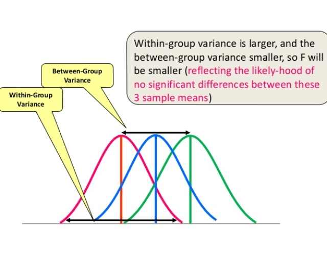
Measures how much the means of each group vary from the mean of the overall population

Within Group Variability

Refers to variations caused by differences within individual groups.

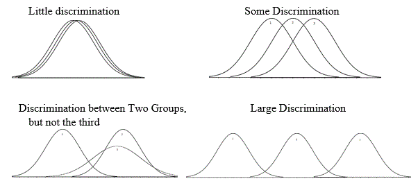
Consider the given distributions of three samples below. As the spread (variability) of each sample is increased, their distributions overlap and they become part of a big population.

Now consider another distribution of the same three samples but with less variability. Although the means of samples are similar to the samples in the above image, they seem to belong to different populations.

Trios:

Take 2 minutes in groups of 3 to discuss which of these following trios would have high f-stats, and which would have low.

Plot them if, if that would help.

Run the f_oneway funciton scypy.stats to check your conclusions

import matplotlib.pyplot as plt
import seaborn as sns
# Create three sets of data without much difference in means
np.random.seed(42)

a = np.random.normal(20,20,20)
b = np.random.normal(22,20,20)
c = np.random.normal(19,20,20)

one = np.random.normal(20,2,20)
two = np.random.normal(22,2,20)
three = np.random.normal(19,2,20)

four = np.random.normal(20,10,20)
five = np.random.normal(20,10,20)
six = np.random.normal(23,10,20)

#__SOLUTION__
fig, ax = plt.subplots(1,3, figsize=(15,10))

sns.distplot(a, hist=False, ax=ax[0])
sns.distplot(b, hist=False, ax=ax[0])
sns.distplot(c, hist=False, ax=ax[0])

sns.distplot(one, hist=False, ax=ax[1])
sns.distplot(two, hist=False, ax=ax[1])
sns.distplot(three, hist=False, ax=ax[1])

sns.distplot(four, hist=False, ax=ax[2])
sns.distplot(five, hist=False, ax=ax[2])
sns.distplot(six, hist=False, ax=ax[2])

# Large variance overcomes the difference in means, so low fstat
print(stats.f_oneway(a,b,c))
# Difference in means is able to overcome the small variance, so high fstat
print(stats.f_oneway(one,two,three))
# Two samples are indistinguishable, but the third sample's large difference in means are able to overcome
# the within group variance to distinguish itself.
print(stats.f_oneway(four,five,six))

F_onewayResult(statistic=0.06693195000987277, pvalue=0.9353322377145488)
F_onewayResult(statistic=11.760064743099003, pvalue=5.2985391195830756e-05)
F_onewayResult(statistic=3.194250788724835, pvalue=0.048432238619556506)

print(stats.f_oneway(a,b,c))
print(stats.f_oneway(one,two,three))
print(stats.f_oneway(four,five,six))

F_onewayResult(statistic=0.06693195000987277, pvalue=0.9353322377145488)
F_onewayResult(statistic=11.760064743099003, pvalue=5.2985391195830756e-05)
F_onewayResult(statistic=3.194250788724835, pvalue=0.048432238619556506)

3. Calculating ANOVA

In this section, we will learn how to calculate ANOVA without using any packages. All we need to calculate is:

$\bar{X} = $ Mean of Means = Mean of entire dataset

Total Sum of Squares is the square of every value minus the mean means, or in other words, the variance of the entire dataset without dividing through by degrees of freedom.

• $SS_t$ = $\sum (X_{ij} - \bar X)^2$

The total sum of squares can be broken down into the sum of squares between and the sum of squares within.

• $SS_t = SS_b+SS_w $

The sum of squares between accounts for variance in the dataset that comes from the difference between the mean of each sample, without dividing through by the degrees of freedom.
Or, in other words, the weighted deviation of each mean from the mean of means:

• $SS_b$ = $\sum(n_i(\bar X - \bar X_i)^2) $

The sum of squares within accounts for variance that comes from within each sample. That is, the sum of the variance of each group weighted by its degrees of freedom. This is really just the sum of the square of each data point's deviation from its sample mean:

• $SS_w$ = $\sum (n_i - 1) s_i ^ 2$

Degrees of Freedom for ANOVA:

• $DF_{between}$ = k - 1
• $DF_{within}$ = N - k
• $DF_{total}$ = N - 1

Notations:

• k is the number of groups

• N is the total number of observations

• n is the number of observations in each group

• $MS_b$ = $\frac{SS_b}{DF_b}$

• $MS_w$ = $\frac{SS_w}{DF_w}$

• $F$ = $\frac{MS_b}{MS_w}$

Like regression and t-test, we can also perform hypothesis testing with ANOVA.

• $H_0$ : $\mu{_1}$ = $\mu_2$ = $\mu_3$ = $\mu_4$
• $H_a$ : $H_0$ is not true

Under the null hypothesis (and with certain assumptions), both quantities estimate the variance of the random error, and thus the ratio should be small. If the ratio is large, then we have evidence against the null, and hence, we would reject the null hypothesis.

import pandas as pd
import scipy.stats as stats
import matplotlib.pyplot as plt
df = pd.read_csv('bikeshare_day.csv')
df.head()
# cnt is the outcome we are trying to predict

<style scoped> .dataframe tbody tr th:only-of-type { vertical-align: middle; }

.dataframe tbody tr th {
    vertical-align: top;
}

.dataframe thead th {
    text-align: right;
}

</style>

	instant	dteday	season	yr	mnth	holiday	weekday	workingday	weathersit	temp	atemp	hum	windspeed	casual	registered	cnt
0	1	2011-01-01	1	0	1	0	6	0	2	0.344167	0.363625	0.805833	0.160446	331	654	985
1	2	2011-01-02	1	0	1	0	0	0	2	0.363478	0.353739	0.696087	0.248539	131	670	801
2	3	2011-01-03	1	0	1	0	1	1	1	0.196364	0.189405	0.437273	0.248309	120	1229	1349
3	4	2011-01-04	1	0	1	0	2	1	1	0.200000	0.212122	0.590435	0.160296	108	1454	1562
4	5	2011-01-05	1	0	1	0	3	1	1	0.226957	0.229270	0.436957	0.186900	82	1518	1600

# we need to conduct a little bit feature engineering to encode 
df['season_cat'] = df.season.apply(lambda x: 'spring' if x == 1 else 
                                           (
                                            'summer' if x == 2 else (
                                                'fall' if x == 3 else 'winter')
                                           )
                                      )
df.head()

<style scoped> .dataframe tbody tr th:only-of-type { vertical-align: middle; }

.dataframe tbody tr th {
    vertical-align: top;
}

.dataframe thead th {
    text-align: right;
}

</style>

	instant	dteday	season	yr	mnth	holiday	weekday	workingday	weathersit	temp	atemp	hum	windspeed	casual	registered	cnt	season_cat
0	1	2011-01-01	1	0	1	0	6	0	2	0.344167	0.363625	0.805833	0.160446	331	654	985	spring
1	2	2011-01-02	1	0	1	0	0	0	2	0.363478	0.353739	0.696087	0.248539	131	670	801	spring
2	3	2011-01-03	1	0	1	0	1	1	1	0.196364	0.189405	0.437273	0.248309	120	1229	1349	spring
3	4	2011-01-04	1	0	1	0	2	1	1	0.200000	0.212122	0.590435	0.160296	108	1454	1562	spring
4	5	2011-01-05	1	0	1	0	3	1	1	0.226957	0.229270	0.436957	0.186900	82	1518	1600	spring

#Create a boxplot
# 1 is spring, 2 is summer, 3 is fall, and 4 is winter
df.boxplot('cnt', by='season_cat', figsize=(6,6))

<matplotlib.axes._subplots.AxesSubplot at 0x1a1f6e04e0>

from scipy import stats
# We could perform two sample t-tests for each sample.

# subset the dataframe  by season and isolate the dependent variable
spring = df[df.season_cat == 'spring'].cnt
fall = df[df.season_cat == 'fall'].cnt
summer = df[df.season_cat == 'summer'].cnt
winter = df[df.season_cat == 'winter'].cnt

# We could run independent t-tests for each combination
# But that increases the chance of making a type I (False Positive) error
# Also, as your groups increase, the number of tests may become infeasable
print(stats.ttest_ind(spring, fall))
print(stats.ttest_ind(spring, summer))
print(stats.ttest_ind(spring, winter ))
print(stats.ttest_ind(fall, summer))
print(stats.ttest_ind(fall, winter))
print(stats.ttest_ind(summer, winter))

Ttest_indResult(statistic=-20.40505135948835, pvalue=2.134072968524431e-62)
Ttest_indResult(statistic=-14.65873026929708, pvalue=1.5284822271363832e-38)
Ttest_indResult(statistic=-12.933694332032188, pvalue=1.2022067175230552e-31)
Ttest_indResult(statistic=3.9765418611661243, pvalue=8.411509811510022e-05)
Ttest_indResult(statistic=5.541003097872063, pvalue=5.7789091515026665e-08)
Ttest_indResult(statistic=1.480020595990678, pvalue=0.13974231789501412)

# Round Robin: 

import numpy as np

mccalister = ['Adam', 'Amanda','Chum', 'Dann', 
 'Jacob', 'Jason', 'Johnhoy', 'Karim', 
'Leana','Luluva', 'Matt', 'Maximilian', ]

np.random.choice(mccalister, 3)

array(['Jacob', 'Karim', 'Adam'], dtype='<U10')

# PSEUDO CODE EXERCISE

1. # Calculate the mean of means.

2. # define a variable (with an appropriate name) which contains the total variability of the dataset, 
# or in other words the total deviation from the mean

3. # define a variable that contains the variability of the dataset which is results from the difference of means.

4. # define a variable that contains the variablity of the dataset which results from the variance of each sample

5. # Sanity Check: make sure all of the variability of the dataset is accounted for by the two last answers.

6. # Define variables that contain the values of the two important degrees of freedom.

7. # Define a variable which holds a value which represents the variance of weighted individual group means.

8. # Define a variable which holds a value which represents the variance of the weighted individual group variances.

9. # Define and properly name a variable whose contents, if close to 1, represents a dataset whose 
# larger group variances drown the distinguishing qualities of differences in means.

9 # Ensure that the prior calculation matches the output below:

f = stats.f_oneway(df['cnt'][df['season_cat'] == 'summer'],
                df['cnt'][df['season_cat'] == 'fall'], 
                df['cnt'][df['season_cat'] == 'winter'],
                df['cnt'][df['season_cat'] == 'spring'])

f.statistic

128.76962156570784

array(['spring', 'summer', 'fall', 'winter'], dtype=object)

#__SOLUTION__
# PSEUDO CODE EXERCISE

1. # Calculate the mean of means.

X_bar = df.cnt.mean()

2. # define a variable (with an appropriate name) which contains the total variability of the dataset, 
# or in other words the total deviation from the mean

ss = sum([(x - X_bar)**2 for x in df.cnt])

3. # define a variable that contains the variability of the dataset which is results from the difference of means.
ssb = sum(
            [len(df[df.season_cat == season])*
             (X_bar 
             - np.mean(df[df.season_cat == season].cnt))**2 
             for season in df.season_cat.unique()
            ])
4. # define a variable that contains the variablity of the dataset which results from the variance of each sample
ssw = sum(
            [(len(df[df.season_cat == season])-1)
             * np.var(df[df.season_cat == season].cnt, ddof=1)
             for season in df.season_cat.unique()
            ])

5. # Sanity Check: make sure all of the variability of the dataset is accounted for by the two last answers.
print(round(ss, 3) == round((ssb + ssw), 3))

6. # Define variables that contain the values of the two important degrees of freedom.
df_b = 4-1
df_w = len(df) - 4


7. # Define a variable which holds a value which represents the variance of weighted individual group means.
msb = ssb/df_b
8. # Define a variable which holds a value which represents the variance of the weighted individual group variances.
msw = ssw/df_w
9. # Define and properly name a variable whose contents, if close to 1, represents a dataset whose 
# larger group variances drown the distinguishing qualities of differences in means.

f_stat = msb/msw

9 # Ensure that the prior calculation matches the output below:

f = stats.f_oneway(df['cnt'][df['season_cat'] == 'summer'],
                df['cnt'][df['season_cat'] == 'fall'], 
                df['cnt'][df['season_cat'] == 'winter'],
                df['cnt'][df['season_cat'] == 'spring'])

round(f.statistic, 3) == round(f_stat, 3)

True





True

4. Calculate ANOVA using statsmodel

data.boxplot('cnt', by = 'season_cat')

<matplotlib.axes._subplots.AxesSubplot at 0x1a269bc940>

from statsmodels.formula.api import ols
import statsmodels.api as sm
# why can we use ols in this case?
anova_season = ols('cnt~season_cat',data=data).fit()
# anova_season.summary()

# examine the anova table 
anova_table = sm.stats.anova_lm(anova_season, type=2)
print(anova_table)

               df        sum_sq       mean_sq           F        PR(>F)
season_cat    3.0  9.505959e+08  3.168653e+08  128.769622  6.720391e-67
Residual    727.0  1.788940e+09  2.460715e+06         NaN           NaN

Perform an ANOVA with scipy

stats.f_oneway(data['cnt'][data['season_cat'] == 'summer'],
                data['cnt'][data['season_cat'] == 'fall'], 
                data['cnt'][data['season_cat'] == 'winter'],
                data['cnt'][data['season_cat'] == 'spring'])

F_onewayResult(statistic=128.76962156570784, pvalue=6.720391362913176e-67)

Next steps

Just because we have rejected the null hypothesis, it doesn't mean we have conclusively showed which group is significantly different from which - remember, the alternative hypothesis is "the null is not true".

We need to conduct post hoc tests for multiple comparison to find out which groups are different, the most prominent post hoc tests are:

• LSD (Least significant difference)
  • $t\sqrt \frac{MSE}{n^2}$
• Tukey's HSD
  • $q\sqrt \frac{MSE}{n}$

https://www.statisticshowto.com/studentized-range-distribution/#qtable

After calculating a value for LSD or HSD, we compare each pair wise mean difference with the LSD or HSD difference. If the pairwise mean difference exceeds the LSD/HSD, then they are significantly different.

from statsmodels.stats.multicomp import pairwise_tukeyhsd
print(pairwise_tukeyhsd(df.cnt, df.season_cat))

    Multiple Comparison of Means - Tukey HSD, FWER=0.05     
============================================================
group1 group2  meandiff  p-adj    lower      upper    reject
------------------------------------------------------------
  fall spring -3040.1706  0.001 -3460.8063 -2619.5349   True
  fall summer  -651.9717  0.001 -1070.8566  -233.0867   True
  fall winter  -916.1403  0.001 -1338.5781  -493.7025   True
spring summer  2388.1989  0.001  1965.3265  2811.0714   True
spring winter  2124.0303  0.001  1697.6383  2550.4224   True
summer winter  -264.1686 0.3792  -688.8337   160.4965  False
------------------------------------------------------------

Two-Way ANOVA:

Using one-way ANOVA, we found out that the season was impactful on the mood of different people. What if the season was to affect different groups of people differently? Say maybe older people were affected more by the seasons than younger people.

Moreover, how can we be sure as to which factor(s) is affecting the mood more? Maybe the age group is a more dominant factor responsible for a person's mode than the season.

For such cases, when the outcome or dependent variable (in our case the test scores) is affected by two independent variables/factors we use a slightly modified technique called two-way ANOVA.

Resources

https://www.analyticsvidhya.com/blog/2018/01/anova-analysis-of-variance/

https://support.minitab.com/en-us/minitab-express/1/help-and-how-to/modeling-statistics/anova/how-to/one-way-anova/before-you-start/overview/