- 如果您在GitHub上在线浏览本页面,强烈建议使用Chrome插件「GitHub with MathJax」来渲染本页面的数学公式。
- Visualizes high-dimensional data by giving each data point a location in a 2 or 3-dimensional map.
- Most of these techniques simply provide tools to display more than two data dimensions, and leave the interpretation of the data to the human observer.
- The aim of dimensionality reduction is to preserve as much of the significant structure of the high-dimensional data as possible in the low-dimensional map.
- 传统的线性技术主要是想让不相似的点在低维表示中分开。
- PCA(Principle Components Analysis,主成分分析)
- MDS(Multiple Dimensional Scaling,多维缩放)
- 对于处于低维、非线性流形上的高维数据而言,更重要的是让相似的近邻点在低维表示中靠近。非线性技术主要保持数据的局部结构。
- Sammon mapping
- CCA(Curvilinear Components Analysis)
- SNE(Stochastic Neighbor Embedding,随机近邻嵌入),t-SNE是基于SNE的。
- Isomap(Isometric Mapping,等度量映射)
- MVU(Maximum Variance Unfolding)
- LLE(Locally Linear Embedding,局部线性嵌入)
- Laplacian Eigenmaps
- In particular, most of the techniques are not capable of retaining both the local and the global structure of the data in a single map.
- In this paper, we introduce
- a way of converting a high-dimensional data set into a matrix of pairwise similarities and,
- a new technique, called “t-SNE”, for visualizing the resulting similarity data.
-
Stochastic Neighbor Embedding,随机近邻嵌入
-
SNE starts by converting the high-dimensional Euclidean distances between datapoints into conditional probabilities that represent similarities.
- 一种基于概率的数据降维处理方法。
- 可以提供原始数据,也可以只提供点之间的相似度,两种输入均可。
-
Given a set of high-dimensional data points
$x_1, x_2, ..., x_n$ ,$p_{i|j}$ is the conditional probability that$x_i$ would pick$x_j$ as its neighbor if neighbors were picked in proportion to their probability density under a Gaussian centered at$x_i$ .$$p_{j|i} = \frac{exp(-||x_i-x_j||^2/2\sigma_i^2)}{\sum_{k\neq i}exp(-||x_i-x_k||^2/2\sigma_i^2)}$$ 注意:1)分母即归一化。2)默认$p_{i|i}=0$。3)每不同数据点$x_i$有不同的$\sigma_i$。其计算方式下面说。
-
Similarly, define
$q_{i|j}$ as conditional probability corresponding to low-dimensional representations of$y_i$ and$y_j$ (corresponding to$x_i$ and$x_j$ ). The variance of Gaussian in this case is set to be$1/\sqrt{2}$ .$$q_{j|i} = \frac{exp(-||y_i-y_j||^2)}{\sum_{k\neq i}exp(-||y_i-y_k||^2)}$$ 注意:若方差取其他值,对结果影响仅仅是缩放而已。
-
If the map points
$y_i$ and$y_j$ correctly model the similarity between the high-dimensional data points$x_i$ and$x_j$ , the conditional probabilities$p_{j|i}$ and$q_{j|i}$ will be equal. -
SNE aims to find a low-dimensional data representation that minimizes the mismatch between
$p_{j|i}$ and$q_{j|i}$ . Thus we use the sum of Kullback-Leibler divergences over all data points as the cost function:$$C=\sum_i KL(P_i||Q_i) = \sum_i \sum_j p_{j|i} log\frac{p_{j|i}}{q_{j|i}}$$ in which
$P_i(k=j)=p_{j|i}$ represents the conditional probability distribution over all other data points given data point$x_i$ .$Q_i(k=j)=q_{j|i}$ too.注意:KLD是不对称的!因为
$KLD=p log(\frac{p}{q})$ ,p>q时为正,p<q时为负。则如果高维数据相邻而低维数据分开(即p大q小),则cost很大;相反,如果高维数据分开而低维数据相邻(即p小q大),则cost很小。所以SNE倾向于保留高维数据的局部结构。 -
对$C$进行梯度下降即可以学习到合适的$y_i$。
The gradient:
$$\frac{\partial C}{\partial y_i} = 2 \sum_j (p_{j|i} - q_{j|i} + p_{i|j} - q_{i|j})(y_i - y_j)$$ and the gradient update with a momentum term:(这里给出但个$y_i$点的梯度下降公式,显然需要对所有$\mathcal{Y}^{(T)}={y_1, y_2, ..., y_n}$进行统一迭代。)
$$y_i^{(t)} = y_i^{(t-1)} + \eta \frac{\partial C}{\partial y_i} + \alpha(t)( y_i^{(t-1)} - y_i^{(t-2)})$$ t-SNE has a cost function that is not convex, i.e. with different initializations we can get different results. 很难优化,也对初值十分敏感,因此要跑多次SNE选取KLD最小/可视化最好结果。(注意这个不是为了泛化,因此选最好的结果即可。)
-
如何为每一个$x_i$选取对应的$\sigma_i$?
-
It is not likely that there is a single value of
$\sigma_i$ that is optimal for all data points in the data set because the density of the data is likely to vary. In dense regions, small$\sigma_i$ , while in sparse region, large$\sigma_i$ . -
Every
$\sigma_i$ is either set by hand (不忍吐槽,原话见于(Hinton and Roweis, 2003)) or found by a simple binary search (Hinton and Roweis, 2003) or by a very robust root-finding method (Vladymyrov and Carreira-Perpinan, 2013) -
使用算法来确定$\sigma_i$要求用户预设困惑度(perplexity)。然后算法找到合适的$\sigma_i$值让条件分布$P_i$的困惑度等于用户预定义的困惑度即可。
$Perp(P_i) = 2^{H(P_i)} = 2^{-\sum_j p_{j|i} log_2 p_{j|i}}$ 注意:困惑度设的大,则显然$\sigma_i$也大。The perplexity increases monotonically with the variance
$\sigma_i$ . -
The perplexity can be interpreted as a smooth measure of the effective number of neighbors. The performance of SNE is fairly robust to changes in the perplexity, and typical values are between 5 and 50.
-
- t-Distributed Stochastic Neighbor Embedding
- SNE有两个问题:
- Cost function 难以优化 -> 解决方案:使用Symmetric SNE。
- Crowding Problem -> 解决方案:在低维嵌入上使用Student's t-distribution替代Guassian distribution,同时也简化了cost function。
-
We define the joint probabilities
$p_{ij}$ in the high-dimensional space to be the symmetrized conditional probabilities, that is, we set$$p_{ij} = \frac{p_{j|i} + p_{i|j}}{2n}$$ -
minimizing the sum of KLD between conditional probabilities -> minimizing a single KLD between joint probability distribution.
$$C = KL(P||Q) = \sum_i \sum_j p_{ij} log \frac{p_{ij}}{q_{ij}}$$ -
The main advantage of the symmetric version of SNE is the simpler form of its gradient, which is faster to compute.
-
$$\frac{\partial C}{\partial y_i} = 4 \sum_j (p_{ij} - q_{ij})(y_i - y_j)$$ (注意:这只是Symmetric SNE的梯度公式,t-SNE的梯度公式类似,推导见后。)
-
“crowding problem”: the area of the two-dimensional map that is available to accommodate moderately distant datapoints will not be nearly large enough compared with the area available to accommodate nearby datapoints.
这句话的意思是:在二维映射空间中,能容纳**(高维空间中的)中等距离间隔点的空间,不会比能容纳(高维空间中的)相近点**的空间大太多。 换言之,哪怕高维空间中离得较远的点,在低维空间中留不出这么多空间来映射。于是到最后高维空间中远的、近的点,在低维空间中统统被塞在了一起,这就叫做“拥挤问题(Crowding Problem)”。
-
Note that the crowding problem is not specific to SNE, but that it also occurs in other local techniques for multidimensional scaling such as Sammon mapping.
-
One way around this problem is to use UNI-SNE (Cook et al. 2007)
这种方法直接给低维空间的点给予一个均匀分布(uniform dist),使得对于高维空间中距离较远的点($p_{ij}$较小),强制保证在低维空间中$q_{ij}>p_{ij}$ (因为均匀分布的两边比高斯分布的两边高出太多了)。
-
Although UNI-SNE usually outperforms standard SNE, the optimization of the UNI-SNE cost function is tedious.
在低维空间中使用均匀分布(UNI-SNE)替代高斯分布(SNE),但cost function优化很复杂,这也是转而使用t分布(t-SNE)取代高斯分布(SNE)的动机。
-
Instead of Gaussian, use a heavy-tailed distribution (like Student-t distribution) to convert distances into probability scores in low dimensions. This way moderate distance in high-dimensional space can be modeled by larger distance in low-dimensional space.
-
-
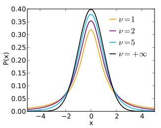
Student's t-distribution has the probability density function given by
$$f(t)={\frac {\Gamma ({\frac {\nu +1}{2}})}{{\sqrt {\nu \pi }},\Gamma ({\frac {\nu }{2}})}}\left(1+{\frac {t^{2}}{\nu }}\right)^{!-{\frac {\nu +1}{2}}}$$ where
$\nu$ is the number of degrees of freedom. -
Special cases
$\nu = 1$ $$f(t) = \frac{1}{\pi (1+t^2)}$$ Called Cauchy distribution. 我们用到是这个简单形式。
-
Special cases
$\nu = \infty$ $$f(t) = \frac{1}{\sqrt{2\pi}} e^{-\frac{t^2}{2}}$$ Called Guassian/Normal distribution.
-
-
-
Why choose t-dist?
- it is closely related to the Gaussian distribution, as the Student t-distribution is an infinite mixture of Gaussians.
- A computationally convenient property is that it is much faster to evaluate the density of a point under a Student t-distribution than under a Gaussian because it does not involve an exponential.
-
Why choose t-dist with single degree of freedom?
-
Because it has particularly nice property: inverse square law. This makes the map’s representation of joint probabilities (almost) invariant to changes in the scale of the map for map points that are far apart. 意思是:这个平方反比的形式,使得当高维空间的两个点再远,他们在低维空间的联合概率几乎不变。结合上一节提到的UNI-SNE:
给低维空间的点给予一个均匀分布(uniform dist),使得对于高维空间中距离较远的点($p_{ij}$较小),强制保证在低维空间中$q_{ij}>p_{ij}$ (因为均匀分布的两边比高斯分布的两边高出太多了)。
从上面的t分布图中可以看到,由于t分布的尾巴高于高斯分布的尾巴,使用t分布同样可以保证对于高维空间中的远距离点,使得在低维空间中$q_{ij}>p_{ij}$。
-
-
The joint probabilities
$q_{ij}$ are defined as$$q_{ij} = \frac{(1 + ||y_i - y_j||^2)^{-1}}{\sum_{k\neq l}(1+||y_k - y_l||^2)^{-1}}$$ (注意:和SNE的$q_{j|i}$公式相比,分母中求和号中,之前是$k\neq i$,表示仅排除$i$自身项;现在是$k\neq l$,表示排除所有自身项 )
-
The cost function is easy to optimize.
$$\frac{\partial C}{\partial y_i} = 4 \sum_j (p_{ij} - q_{ij})(y_i - y_j)(1+ ||y_i - y_j||^2)^{-1}$$ (注意:是在Symmetric SNE的梯度公式后面加上了$(1+ ||y_i - y_j||^2)^{-1}$一项,推导见论文附录A。)
- Space and time complexity is quadratic ($O(n^2)$) in the number of datapoints so infeasible to apply on large datasets.
- Random walk
- Select a random subset of points (called landmark points) to display.
- for each landmark point, define a random walk starting at a landmark point and terminating at any other landmark point.
-
$p_{i|j}$ is defined as fraction of random walks starting at$x_i$ and finishing at$x_j$ (both these points are landmark points). This way,$p_{i|j}$ is not sensitive to "short-circuits" in the graph (due to noisy data points).
-
Barnes-Hut approximations (Van Der Maaten, 2014)
- allowing it to be applied on large real-world datasets. We applied it on data sets with up to 30 million examples.
- Gaussian kernel employed by t-SNE (in high-dimensional) defines a soft border between the local and global structure of the data.
- Both nearby and distant pair of datapoints get equal importance in modeling the low-dimensional coordinates.
- The local neighborhood size of each datapoint is determined on the basis of the local density of the data.
- Random walk version of t-SNE takes care of "short-circuit" problem.
- it is unclear how t-SNE performs on general dimensionality reduction tasks,
- the relatively local nature of t-SNE makes it sensitive to the curse of the intrinsic dimensionality of the data, and
- t-SNE is not guaranteed to converge to a global optimum of its cost function.
-
关于SNE的梯度公式
$$\frac{\partial C}{\partial y_i} = 2 \sum_j (p_{j|i} - q_{j|i} + p_{i|j} - q_{i|j})(y_i - y_j)$$ 作者在论文第4页用了一个弹簧的比喻来解释,如图:

可以把该公式看做是所有$y_j$通过弹簧(图中箭头)对$y_i$的合力,类比胡克定律$F=k\Delta x$,这里$(y_i - y_j)$表示拉伸长度,而$(p_{j|i} - q_{j|i} + p_{i|j} - q_{i|j})$表示弹性系数。表示高维数据点和低维映射点之间点相似度的失配程度(mismatch between the pairwise similarities of the data points and the map points)。按这么来说,弹性系数应该写成$(\frac{p_{j|i} + p_{i|j}}{2} - \frac{q_{j|i} + q_{i|j}}{2})$的形式,有趣的是,如果写成这种形式,则SNE、Symmetric SNE、t-SNE的梯度公式形式上就统一了。
Gradient SNE $\frac{\partial C}{\partial y_i} = 4 \sum_j (\frac{p_{j Symmetric SNE $\frac{\partial C}{\partial y_i} = 4 \sum_j (p_{ij} - q_{ij})(y_i - y_j)$ t-SNE $\frac{\partial C}{\partial y_i} = 4 \sum_j (p_{ij} - q_{ij})(y_i - y_j)(1+
