Governing equation for the contrast agent concentration

[iMTimmyyy]

Dear @lululxvi,

Hi I am trying to model and solve the following equation :

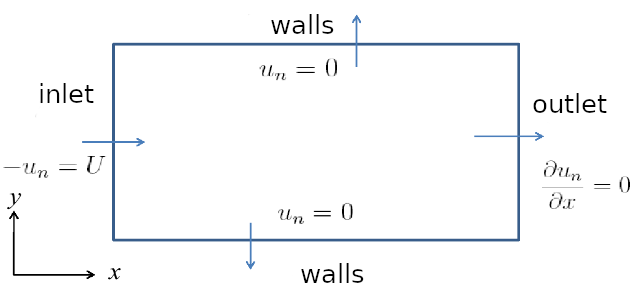
over a rectangle domain like this (20mm by 2mm):

where there are zero-gradient boundary conditions at the upper, lower walls and outlet and a Dirichlet boundary condition at the inlet for the concentration. And for initial condition, it is zero everywhere. And velocity is 0.2 m/s in the x-direction

And my script is as follow:

from future import absolute_import
from future import division
from future import print_function

import matplotlib.pyplot as plt
import numpy as np
import deepxde as dde
from deepxde.backend import tf

def main():

def pde(x, y):
    dy_x = tf.gradients(y, x)[0]
    dy_x, dy_y, dy_t = dy_x[:, 0:1], dy_x[:, 1:2], dy_x[:, 2:]
    dy_xx = tf.gradients(dy_x, x)[0][:, 0:1]
    dy_yy = tf.gradients(dy_y, x)[0][:, 1:2]
    return dy_t + 0.2 * dy_x - 0.01 * (dy_xx + dy_yy)

def boundary_l(x, on_boundary):
    return on_boundary and np.isclose(x[0], 0)

def boundary_r(x, on_boundary):
    return on_boundary and np.isclose(x[0], 20e-3)

def boundary_up(x, on_boundary):
    return on_boundary and np.isclose(x[1], 2e-3)

def boundary_low(x, on_boundary):
    return on_boundary and np.isclose(x[1], 0)

def func_zero(x):
    return np.zeros((len(x), 1))

def func_one(x):
    return np.ones((len(x), 1))

def func(x):
    return np.sin(x[:, 2:]/0.005)**2

geom = dde.geometry.Rectangle(xmin=[0, 0], xmax=[20e-3, 2e-3])
timeDomain = dde.geometry.TimeDomain(0, 0.5)
geomtime = dde.geometry.GeometryXTime(geom, timeDomain)

bc_l = dde.DirichletBC(geomtime, func, boundary_l)
bc_r = dde.NeumannBC(geomtime, func_zero, boundary_r)
bc_up = dde.NeumannBC(geomtime, func_zero, boundary_up)
bc_low = dde.NeumannBC(geomtime, func_zero, boundary_low)
ic = dde.IC(geomtime, func_zero, lambda _, on_initial: on_initial)

data = dde.data.TimePDE(
    geomtime, pde, [bc_l, bc_r, bc_up, bc_low, ic], num_domain=5000, num_boundary=10000,  num_initial=150)

layer_size = [3] + [50] * 4 + [1]
activation_func = "tanh"
initializer = "Glorot uniform"

net = dde.maps.FNN(layer_size, activation_func, initializer)
model = dde.Model(data, net)

model.compile("adam", lr=1.5e-3)
model.train(epochs=30000)
model.compile("L-BFGS-B")
losshistory, train_state = model.train(model_save_path=r"C:\Users\timmy\PycharmProjects\examples\New\sin5D10Bdot5")
dde.saveplot(losshistory, train_state, issave=False, isplot=True)

if name == "main":
main()

Originally, I was using a fixed value for the Dirichlet condition (func_one, 5000 Domain and 3000 boundary points) and it worked fine. However, when I changed the Dirichlet condition to sin^2(t/0.005), it behaved strangely. The test loss is much lower than train loss (e.g. train loss: 1e-1, test loss: 1e-4/-5) and the prediction I obtained is very different from numerical solutions.

The Prediction:

Numerical Solutions:

Besides, when I tried to add the "num_test" argument in TimePDE I got the following error:

Traceback (most recent call last):
File "C:/Users/timmy/PycharmProjects/examples/CA_Conc.py", line 111, in
main()
File "C:/Users/timmy/PycharmProjects/examples/CA_Conc.py", line 51, in main
geomtime, pde, [bc_l, bc_r, bc_up, bc_low, ic], num_domain=5000, num_boundary=3000, num_initial=150, num_test=1000)
File "C:\Users\timmy\AppData\Roaming\Python\Python37\site-packages\deepxde\data\pde.py", line 162, in init
num_test=num_test,
File "C:\Users\timmy\AppData\Roaming\Python\Python37\site-packages\deepxde\data\pde.py", line 45, in init
self.test()
File "C:\Users\timmy\AppData\Roaming\Python\Python37\site-packages\deepxde\utils.py", line 23, in wrapper
return func(self, *args, **kwargs)
File "C:\Users\timmy\AppData\Roaming\Python\Python37\site-packages\deepxde\data\pde.py", line 89, in test
self.test_x = self.test_points()
File "C:\Users\timmy\AppData\Roaming\Python\Python37\site-packages\deepxde\data\pde.py", line 191, in test_points
return self.geom.uniform_points(self.num_test)
File "C:\Users\timmy\AppData\Roaming\Python\Python37\site-packages\deepxde\geometry\timedomain.py", line 53, in uniform_points
nt = int(np.ceil(n / nx))
ZeroDivisionError: division by zero

Process finished with exit code 1

And I got this error when I tried to add metrics = ["l2 relative error"] to model.complie("adam", lr=1.5e-3):
File "C:\Users\timmy\AppData\Roaming\Python\Python37\site-packages\deepxde\metrics.py", line 15, in l2_relative_error
return np.linalg.norm(y_true - y_pred) / np.linalg.norm(y_true)
TypeError: unsupported operand type(s) for -: 'NoneType' and 'float'

Could you help me identify what might be wrong?
Thank you in advance.

[lululxvi]

• The train loss includes all the loss terms, and the test loss only includes the PDE loss. Your train loss is large, and I suspect the IC loss term is large. You can check each loss term, and find out which one is large.
• Try a small time domain firs, e.g., (0, 0.1), more training points, longer training
• num_test you used may be too small
• You need to pass the reference solution to the solution argument to compute "l2 relative error"

[iMTimmyyy]

• The train loss includes all the loss terms, and the test loss only includes the PDE loss. Your train loss is large, and I suspect the IC loss term is large. You can check each loss term, and find out which one is large.
• Try a small time-domain firs, e.g., (0, 0.1), more training points, longer training
• num_test you used may be too small
• You need to pass the reference solution to the solution argument to compute "l2 relative error"

Thank you for your quick reply @lululxvi

So I tried your suggestions and interestingly when I reduced the time domain from 0.5s to 0.1s, the prediction became worse (normally, it should get better right? Since the density of collocation points further increases)!

I also tried to use more training points (15000 domain and boundary points, 5000 initial condition points) but my train and test loss graphs of different trainings (I tried to use training points ranged from 5000 to 15000).stay pretty similar (just flatten up).

Additionally, I thought it has something to do with the complexity of the model and the learning rate, so I tried to use a different network size ( [40]*6 and using learning rate 1.5e-3 and 3e-3) but it didn't get any better.

Do you think I should keep using more training points, longers training and further increasing the complexity of the model?

The following losses are from one of my training, do you reckon my number of initial condition points is not enough?
Step Train loss Test loss Test metric
0 [4.66e-02, 3.71e-01, 2.86e-02, 4.61e-04, 4.61e-04, 3.88e-06] [4.66e-02, 0.00e+00, 0.00e+00, 0.00e+00, 0.00e+00, 0.00e+00] []
1000 [1.30e-04, 1.81e-01, 2.72e-05, 3.76e-06, 3.71e-06, 5.90e-02] [1.30e-04, 0.00e+00, 0.00e+00, 0.00e+00, 0.00e+00, 0.00e+00] []
2000 [1.44e-04, 1.81e-01, 2.32e-05, 1.60e-08, 1.57e-08, 5.90e-02] [1.44e-04, 0.00e+00, 0.00e+00, 0.00e+00, 0.00e+00, 0.00e+00] []
3000 [3.30e-05, 1.83e-01, 6.43e-05, 7.72e-04, 7.70e-04, 5.79e-02] [3.30e-05, 0.00e+00, 0.00e+00, 0.00e+00, 0.00e+00, 0.00e+00] []
4000 [1.44e-04, 1.81e-01, 2.33e-05, 2.29e-08, 2.26e-08, 5.90e-02] [1.44e-04, 0.00e+00, 0.00e+00, 0.00e+00, 0.00e+00, 0.00e+00] []
5000 [1.73e-04, 1.81e-01, 2.35e-05, 1.07e-07, 1.04e-07, 5.90e-02] [1.73e-04, 0.00e+00, 0.00e+00, 0.00e+00, 0.00e+00, 0.00e+00] []
6000 [1.26e-04, 1.82e-01, 4.19e-05, 3.39e-07, 3.40e-07, 5.86e-02] [1.26e-04, 0.00e+00, 0.00e+00, 0.00e+00, 0.00e+00, 0.00e+00] []
7000 [1.64e-04, 1.81e-01, 2.36e-05, 1.77e-08, 1.65e-08, 5.90e-02] [1.64e-04, 0.00e+00, 0.00e+00, 0.00e+00, 0.00e+00, 0.00e+00] []
8000 [1.16e-04, 1.82e-01, 2.24e-05, 9.99e-09, 9.67e-09, 5.84e-02] [1.16e-04, 0.00e+00, 0.00e+00, 0.00e+00, 0.00e+00, 0.00e+00] []
9000 [1.44e-04, 1.81e-01, 2.30e-05, 1.02e-08, 1.01e-08, 5.90e-02] [1.44e-04, 0.00e+00, 0.00e+00, 0.00e+00, 0.00e+00, 0.00e+00] []
10000 [1.44e-04, 1.81e-01, 2.33e-05, 1.03e-08, 1.03e-08, 5.90e-02] [1.44e-04, 0.00e+00, 0.00e+00, 0.00e+00, 0.00e+00, 0.00e+00] []
11000 [1.44e-04, 1.81e-01, 2.33e-05, 1.04e-08, 1.04e-08, 5.90e-02] [1.44e-04, 0.00e+00, 0.00e+00, 0.00e+00, 0.00e+00, 0.00e+00] []
12000 [1.44e-04, 1.81e-01, 2.33e-05, 1.03e-08, 1.03e-08, 5.90e-02] [1.44e-04, 0.00e+00, 0.00e+00, 0.00e+00, 0.00e+00, 0.00e+00] []
13000 [1.44e-04, 1.81e-01, 2.32e-05, 1.02e-08, 1.02e-08, 5.90e-02] [1.44e-04, 0.00e+00, 0.00e+00, 0.00e+00, 0.00e+00, 0.00e+00] []
14000 [1.44e-04, 1.81e-01, 2.32e-05, 1.02e-08, 1.01e-08, 5.89e-02] [1.44e-04, 0.00e+00, 0.00e+00, 0.00e+00, 0.00e+00, 0.00e+00] []
15000 [1.44e-04, 1.81e-01, 2.33e-05, 1.03e-08, 1.03e-08, 5.90e-02] [1.44e-04, 0.00e+00, 0.00e+00, 0.00e+00, 0.00e+00, 0.00e+00] []
16000 [3.40e-04, 1.79e-01, 3.69e-05, 4.06e-07, 4.05e-07, 6.15e-02] [3.40e-04, 0.00e+00, 0.00e+00, 0.00e+00, 0.00e+00, 0.00e+00] []
17000 [1.44e-04, 1.81e-01, 2.33e-05, 1.03e-08, 1.02e-08, 5.90e-02] [1.44e-04, 0.00e+00, 0.00e+00, 0.00e+00, 0.00e+00, 0.00e+00] []
18000 [1.44e-04, 1.81e-01, 2.34e-05, 1.04e-08, 1.04e-08, 5.90e-02] [1.44e-04, 0.00e+00, 0.00e+00, 0.00e+00, 0.00e+00, 0.00e+00] []
19000 [1.44e-04, 1.81e-01, 2.33e-05, 1.03e-08, 1.03e-08, 5.90e-02] [1.44e-04, 0.00e+00, 0.00e+00, 0.00e+00, 0.00e+00, 0.00e+00] []
20000 [1.44e-04, 1.81e-01, 2.33e-05, 1.03e-08, 1.03e-08, 5.90e-02] [1.44e-04, 0.00e+00, 0.00e+00, 0.00e+00, 0.00e+00, 0.00e+00] []
21000 [1.46e-04, 1.81e-01, 2.43e-05, 1.06e-08, 1.06e-08, 5.91e-02] [1.46e-04, 0.00e+00, 0.00e+00, 0.00e+00, 0.00e+00, 0.00e+00] []
22000 [1.44e-04, 1.81e-01, 2.33e-05, 1.03e-08, 1.03e-08, 5.90e-02] [1.44e-04, 0.00e+00, 0.00e+00, 0.00e+00, 0.00e+00, 0.00e+00] []
23000 [1.44e-04, 1.81e-01, 2.34e-05, 1.04e-08, 1.05e-08, 5.90e-02] [1.44e-04, 0.00e+00, 0.00e+00, 0.00e+00, 0.00e+00, 0.00e+00] []
24000 [1.14e-04, 1.81e-01, 1.94e-05, 1.77e-08, 1.71e-08, 5.89e-02] [1.14e-04, 0.00e+00, 0.00e+00, 0.00e+00, 0.00e+00, 0.00e+00] []
25000 [1.44e-04, 1.81e-01, 2.32e-05, 1.02e-08, 1.02e-08, 5.90e-02] [1.44e-04, 0.00e+00, 0.00e+00, 0.00e+00, 0.00e+00, 0.00e+00] []
26000 [1.44e-04, 1.81e-01, 2.32e-05, 1.02e-08, 1.02e-08, 5.90e-02] [1.44e-04, 0.00e+00, 0.00e+00, 0.00e+00, 0.00e+00, 0.00e+00] []
27000 [1.36e-04, 1.81e-01, 2.36e-05, 1.05e-08, 1.05e-08, 5.90e-02] [1.36e-04, 0.00e+00, 0.00e+00, 0.00e+00, 0.00e+00, 0.00e+00] []
28000 [1.44e-04, 1.81e-01, 2.33e-05, 1.03e-08, 1.03e-08, 5.90e-02] [1.44e-04, 0.00e+00, 0.00e+00, 0.00e+00, 0.00e+00, 0.00e+00] []
29000 [1.45e-04, 1.81e-01, 2.31e-05, 1.13e-08, 1.12e-08, 5.90e-02] [1.45e-04, 0.00e+00, 0.00e+00, 0.00e+00, 0.00e+00, 0.00e+00] []
30000 [8.48e-05, 1.81e-01, 2.48e-05, 6.18e-08, 6.17e-08, 5.90e-02] [8.48e-05, 0.00e+00, 0.00e+00, 0.00e+00, 0.00e+00, 0.00e+00] []

[lululxvi]

The loss is too large. Check "Q: I failed to train the network or get the right solution, e.g., the training loss is large." at FAQ.

[iMTimmyyy]

Hi lulu,

I have sort of figured out how to solve my problem by adjusting the ratio of my number of domain, boundary and initial condition point and using the argument loss_weights in model.compile.

Thank you for making this awesome deep learning library.

[katayooneshkofti]

@iMTimmyyy is it possible to upload your final code?

[iMTimmyyy]

@iMTimmyyy is it possible to upload your final code?

Sure, here you go.

`from future import absolute_import
from future import division
from future import print_function

import matplotlib.pyplot as plt
import numpy as np
import deepxde as dde
from deepxde.backend import tf

def main():

def pde(x, y):
    dy_x = tf.gradients(y, x)[0]
    dy_x, dy_y, dy_t = dy_x[:, 0:1], dy_x[:, 1:2], dy_x[:, 2:]
    dy_xx = tf.gradients(dy_x, x)[0][:, 0:1]
    dy_yy = tf.gradients(dy_y, x)[0][:, 1:2]
    return dy_t + 0.2 * dy_x - 0.01 * (dy_xx + dy_yy)

def boundary_l(x, on_boundary):
    return on_boundary and np.isclose(x[0], 0)

def boundary_r(x, on_boundary):
    return on_boundary and np.isclose(x[0], 20e-3)

def boundary_up(x, on_boundary):
    return on_boundary and np.isclose(x[1], 2e-3)

def boundary_low(x, on_boundary):
    return on_boundary and np.isclose(x[1], 0)

def func_zero(x):
    return np.zeros((len(x), 1))

def func_one(x):
    return np.ones((len(x), 1))

def func(x):
    return np.sin(x[:, 2:3]/0.005)**2

geom = dde.geometry.Rectangle(xmin=[0, 0], xmax=[20e-3, 2e-3])
timeDomain = dde.geometry.TimeDomain(0, 0.1)
geomtime = dde.geometry.GeometryXTime(geom, timeDomain)

bc_l = dde.DirichletBC(geomtime, func, boundary_l)
bc_r = dde.NeumannBC(geomtime, func_zero, boundary_r)
bc_up = dde.NeumannBC(geomtime, func_zero, boundary_up)
bc_low = dde.NeumannBC(geomtime, func_zero, boundary_low)
ic = dde.IC(geomtime, func_zero, lambda _, on_initial: on_initial)

data = dde.data.TimePDE(
    geomtime, pde, [bc_l, bc_r, bc_up, bc_low, ic], num_domain=10000, num_boundary=15000,  num_initial=3300)

layer_size = [3] + [60] * 4 + [1]
activation_func = "tanh"
initializer = "Glorot uniform"

net = dde.maps.FNN(layer_size, activation_func, initializer)
model = dde.Model(data, net)

model.compile("adam", lr=1e-3, loss_weights=[1, 60, 1, 1, 1, 1])
model.train(epochs=50000)
model.compile("L-BFGS-B", loss_weights=[1, 60, 1, 1, 1, 1])
losshistory, train_state = model.train(model_save_path=r"C:\Users\timmy\PycharmProjects\examples\60-4_sin\10D15B3C60wdot1")`

[katayooneshkofti]

@iMTimmyyy Thank you
did you find these weights by trial and error?