- Check results visually to ensure reads align to expected regions without excess mismatches.
- Genome browsers give a linear track representing the forward stand of the genome. left = 5'. right = 3'
- Visualise in line orientated formats (fasta, bed, gff, SAM/BAM)
- genomic features are drawn over the linear track in glyphs (pictogram)
- Horizontal intervals = directions, genes, alignments
- Values over intervals = coverages, probabilities
- Attributes at locations = mutations, deletions, junctions
- To create publication genome browser shots, merge bedgraphs for each group, then upload tracks to UCSC genome browser > download
- simplest genome browser. can visualise any DAM file
samtools tview --reference reference_genome.fa filename.bam
- Integrative Genomics Viewer IGV by the Broad Institute
- Integrated Genome Browser IGB by University of North Carolina
- Artemis by the Wellcome Sanger Institute
- Tablet by James Hutton Institute
- SeqMonk for high throughput RNA-seq
- iobio for real-time genomic analysis
Convert BAM > BigWig file using BED tools & BED graph. Can then import the BigWig file into IGV & UCSC genome browsers. STAR creates a wiggle track (raw bigwig file). They only show the coverage and not the individual reads. They are binary formatted and so a much smaller files - prevents IGV crashing.
https://software.broadinstitute.org/software/igv/bigwig https://github.com/YangLab/bamTobw
Use bamCoverage to convert BAM > BW files
ml STAR

#set bam input
BAM=/home/camp/ziffo/working/oliver/projects/vcp_fractionation/alignment/roi_bam/*.bam
#set OUT directory
OUT=/camp/home/ziffo/working/oliver/projects/vcp_fractionation/alignment/roi_bam/BigWigs

for SAMPLE in $BAM
do
	sbatch -N 1 -c 4 --mem=24GB --wrap="STAR --runMode inputAlignmentsFromBAM --runThreadN 24 --inputBAMfile $SAMPLE --outWigType wiggle --outWigStrand Unstranded --outWigNorm RPM --outFileNamePrefix $SAMPLE"
doneBest resources are the IVG mannual and youtube videos https://www.biostarhandbook.com/visualize/igv.html
- Run IGV on local computer and mount CAMP. Set Java 8 as default since IGV doesnt work with Java 10
# On local terminal move to IGV in bin
cd ~/bin/IGV_2.4.14/lib
# run IGV via command line on local terminal
java -Xmx750m -jar igv.jar- Set reference genome to Human (hg38) top left box.
- Click File load from file > click Desktop > mount CAMP locally > click relevant BigWig (.bw) or BAM files (to see individual read tracks) files (load multiple at once).
To visualise on IGV its easier to generate TDF files which are much lighter. This is useful if want to add more data-sets later. To generate TDF files first generate Bedgraph coverage files, then sort and then create the tdf file. Create 3 different coverage files: positive, negative strands and total. As the data is stranded it is better to look at both strands separately. Run the code in file: PE_strandedBedGraph.sh
-
Rename BAM files: right click file name in left hand column.
-
Go to the Genomic Location of interest: search gene name or gene coordinates e.g. SFPQ or chr1:35,176,378-35,193,158 in top middle box > Go. Find Genomic Locations using google search eg https://www.genecards.org/cgi-bin/carddisp.pl?gene=SFPQ Mark the region of interest: Regions > Region Navigator > Add
-
Zoom in & out using top right zoomer or +/-. IGV will ask you to zoom in to see alignment data. This is because it has a default of 30 kb memory. You can change this to a higher value to see alignment data from a further out zoom but this will slow down the processing speed when scrolling across the genome. If you have deep coverage files then keep memory low to avoid it slowing down processing.
For each BAM file there are 2 tracks. Top track shows summary distribution of the coverage of the exonic islands separated by spice junctions (introns). Bottom tracks show all the individual sequence read alignments piled up.
- Compare exon usage in the top tracks to transcript genome (bottom row): make the rows for each of the BAM files smaller and right click on the reference genome at the bottom row (in blue) > expand to show all the previously annotated differential splicing.
Bases that dont match the reference sequences are highlighted by colour. The deeper the shade of grey the more confidence you can have that the sequence was aligned correctly. White means no confidence alignment.

IGV is used only to validate & confirm analysis results. Use it to explore large genomic datasets. It is not good for the primary analysis.

Top row = chromosome. red bar is location. blue lines mid-section refer to transcripts binding with more = higher peak. bottom section = reference genomes. Coverage line = quick identification of highly covered regions Grey boxes = aligned reads. Gaps between reads with horizontal grey line = introns Blue lines within reads = insertions Red lines within reads = deletions Blue boxes = reference genome
Short introduction to UCSC genome browser PDF http://genome.ucsc.edu/training/index.html https://www.youtube.com/channel/UCQnUJepyNOw0p8s2otX4RYQ https://www.sciencedirect.com/science/article/pii/S0888754308000451?via%3Dihub http://genome.ucsc.edu/goldenPath/help/hgTracksHelp.html
Upload merged bigwig files to genome browser to download figures for publication.
- Merge BAM files for each group takes 10mins
ml SAMtools
ml STAR
# VCP NPC D7
sbatch -N 1 -c 4 --mem=24GB --wrap="samtools merge VCP_NPC_D7_merged.bam SRR5483788_Aligned.sortedByCoord.out.bam SRR5483789_Aligned.sortedByCoord.out.bam SRR5483790_Aligned.sortedByCoord.out.bam"
# VCP iPSC D0
sbatch -N 1 -c 4 --mem=24GB --wrap="samtools merge VCP_iPSC_D0_merged.bam SRR5483800Aligned.sortedByCoord.out.bam SRR5483801Aligned.sortedByCoord.out.bam SRR5483802Aligned.sortedByCoord.out.bam"

# index merged BAMs
sbatch -N 1 -c 8 --mem 40 --wrap="samtools index VCP_NPC_D7_merged.bam"
sbatch -N 1 -c 8 --mem 40 --wrap="samtools index VCP_iPSC_D0_merged.bam"- Convert merged BAMs > BigWig & normalise for read depth
sbatch -N 1 -c 4 --mem=24GB --wrap="STAR --runMode inputAlignmentsFromBAM --runThreadN 24 --inputBAMfile VCP_NPC_D7_merged.bam --outWigType wiggle --outWigStrand Unstranded --outWigNorm RPM --outFileNamePrefix VCP_NPC_D7_merged"

sbatch -N 1 -c 4 --mem=24GB --wrap="STAR --runMode inputAlignmentsFromBAM --runThreadN 24 --inputBAMfile VCP_iPSC_D0_merged.bam --outWigType wiggle --outWigStrand Unstranded --outWigNorm RPM --outFileNamePrefix VCP_iPSC_D0_merged"Click + in top right of screen Click Binary Choose Files > select merged bigWig files Edit the track - remove unwanted tracks, go to relevant genes
Alternatives are to upload to UCSC - couldnt get this to work as bigWigs too large. See page 13 here Login to UCSC browser: MyData > MySessions > Login http://genome.ucsc.edu/cgi-bin/hgSession?hgsid=733417633_FrgAYw50hwa3PWBTCps2DLCXaSLK&hgS_doMainPage=1 Click Genome Browser in Menu. Check reference genome is hg38 Enter gene of interest in search box > click track of interest Click Add custom track, next to the bottom box click upload, on CAMP select the merged.bw file - allow time for upload
Or use ggbio in Rstudio http://bioconductor.org/packages/release/bioc/vignettes/ggbio/inst/doc/ggbio.pdf
-
Download or screenshot
-
Finalise in Illustrator
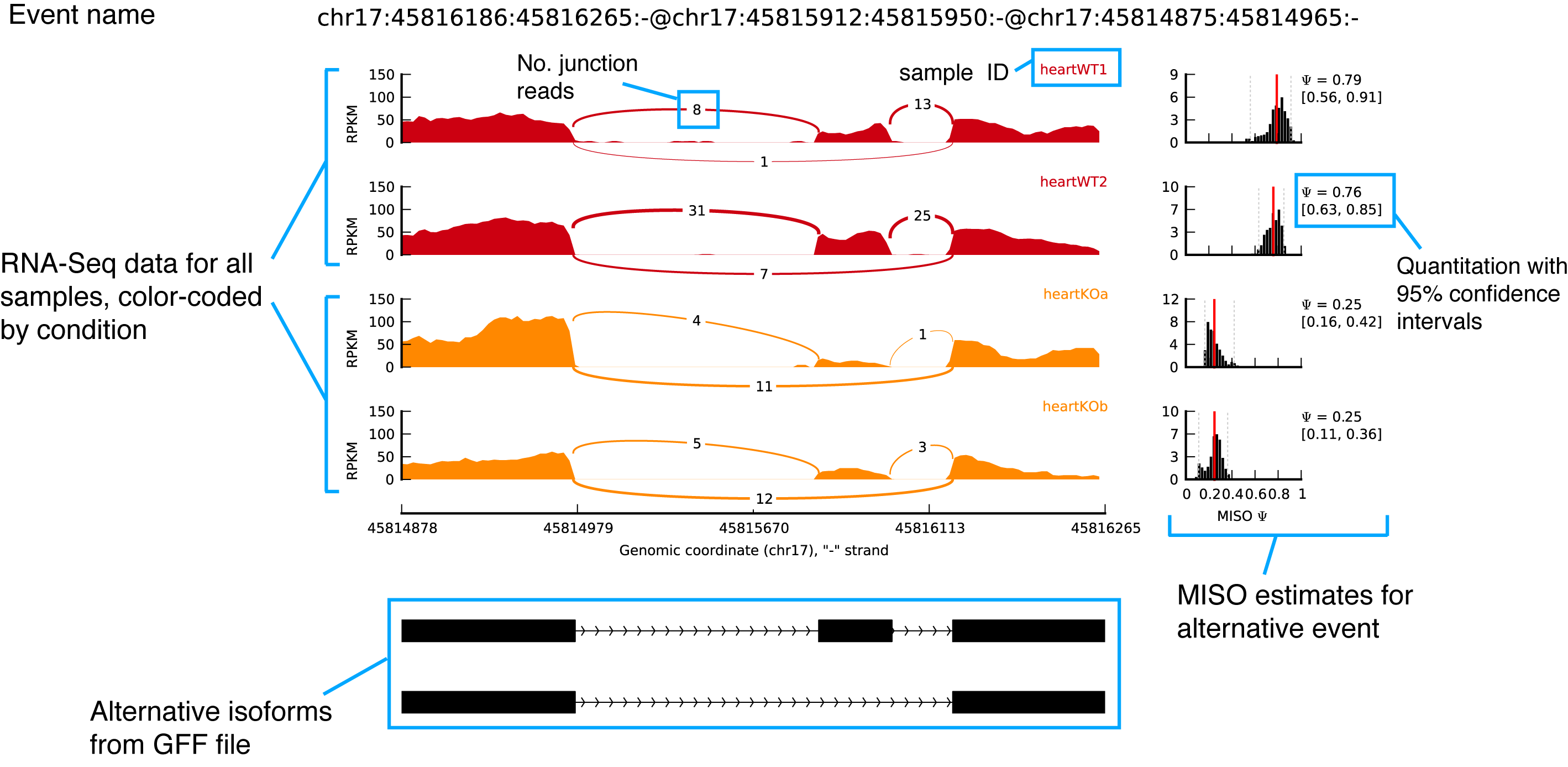
Sashimi Plots
Visualise splice junctions & explore exon usage
Follow instructions in this video: https://www.youtube.com/watch?v=UvHihNbyCh8
Create a public link to a UCSC genome browser session displaying the uploaded sequence tracks: https://genome.ucsc.edu/cgi-bin/hgGateway
Instructions are available here http://genome.ucsc.edu/goldenPath/help/hgSessionHelp.html#NAR
BAM > bigwigs
https://deeptools.readthedocs.io/en/develop/content/tools/bamCoverage.html
module load Anaconda3
python -m venv /camp/home/ziffo/home/envs
source /camp/home/ziffo/home/envs/bin/activate
python -m pip install deeptools

# For merged BAM files:
cd /camp/home/ziffo/home/projects/inter-neuron-bulk-rnaseq/alignment/STAR/merged
sbatch -N 1 -c 10 --mem=40G -t 48:00:00 --wrap="bamCoverage -b in_d18_ctrl.bam -o in_d18_ctrl.bw" --mail-type=ALL,ARRAY_TASKS --mail-user=oliver.ziff@crick.ac.uk --job-name=bamCoverage --output=bamCoverage-%j.out --error=bamCoverage-%j.err
Convert GTF > BED > bigBed format
Move files to shareable location (Dropbox) and make shareable with others
cd /Users/ziffo/'Dropbox (The Francis Crick)'/Medical\ Files/Research/PhD/projects/inter-neuron-bulk-rnaseq/bigWigs
rsync -aP camp-ext:/camp/home/ziffo/home/projects/inter-neuron-bulk-rnaseq/alignment/STAR/merged/*.bw .
Create link > Copy link > paste into track lines script
track type=bigWig name="IN D18" description="interneuron day 18 control" color=0,0,255 visibility=2 bigDataUrl=https://www.dropbox.com/s/g7bond1pr88xqym/in_d18_ctrl.bw?dl=1
track type=bigWig name="IN D25" description="interneuron day 25 control" color=255,0,0 visibility=2 bigDataUrl=https://www.dropbox.com/s/jt18a30ik9qz5zk/in_d25_ctrl.bw?dl=1
track type=bigWig name="MN D18" description="motor neuron day 18 control" color=0,0,255 visibility=2 bigDataUrl=https://www.dropbox.com/s/jvyrath43s7kp33/mn_d18_ctrl.bw?dl=1
track type=bigWig name="MN D25" description="motor neuron day 25 control" color=255,0,0 visibility=2 bigDataUrl=https://www.dropbox.com/s/rsn2waae8m8mi6z/mn_d25_ctrl.bw?dl=1
track type=BED name="annotation" description="GENCODE annotation" color=0,255,0 visibility=3 bigDataUrl=https://www.dropbox.com/s/ke2ddj4zwl6bs74/Human.GRCh38.GENCODEv24.bed?dl=1
Ensure dropbox link is dl=1 at end
Login to UCSC
Reset user settings http://genome.ucsc.edu/cgi-bin/cartReset
Configure genome browser http://genome.ucsc.edu/cgi-bin/hgTracks?hgsid=968366871_acZUce1tkq5mADRGXsXv022MGtG8
Add custom tracks
In top box > paste the track lines settings into box > submit
Save as a new UCSC session: http://genome.ucsc.edu/cgi-bin/hgSession?hgsid=968355787_90NOUDSzGcMJd8jgzNvA2TiOUEW2&hgS_doMainPage=1
After creating your custom tracks and viewing your data on the Genome Browser, you can save all of your tracks and settings to a snapshot of the Genome Browser called a session. You can easily save a session by following these five steps:
- Configure the Genome Browser to your preference
Make sure the display of your custom tracks is to your liking on the Genome Browser. - Navigate to the sessions page
Once you are satisfied with the display, go to the My Sessions page by either:- Going to My Data -> My Sessions from the navigation bar.
- Using the "s then s" keyboard shortcut when viewing the main page of the Genome Browser.
- Login to the UCSC Genome Browser
You must sign in to be able to save named sessions which will then be displayed with Browser and Email links. - Save your session
Go to the Save Settings section and in the Save current settings as named session text box, enter a name for your session. When saving the session, be sure to have the "allow this session to be loaded by others" option checked and then click submit. - Edit the session description
Once the session is created, you can click the details button to add a description to the session. If you eventually make a Public Session, and provide a detailed description, anyone can find it by searching for terms you share. For example, navigate to the Public Sessions page and search "NAR" to see some example sessions.