Large W Limit of Knapsack Problem

Motivation for statistical-physics algorithm

The Knapsack Problem is a classic problem from combinatorial optimization. In the "0-1" version of the problem, we are given N objects each of which has a value and a weight, and our objective is to find the collection of objects that maximizes the total value of the collection while ensuring that the weight remain under a given maximum.

This repository contains code for an algorithm that solves this "0-1" problem in the limit where the weight W is large.

We compare this algorithm with other exact algorithms for the knapsack problem (RossettaCode Knapsack), which generally proceed in more time. The code and figures in this repository were used to produce the results in the associated paper.

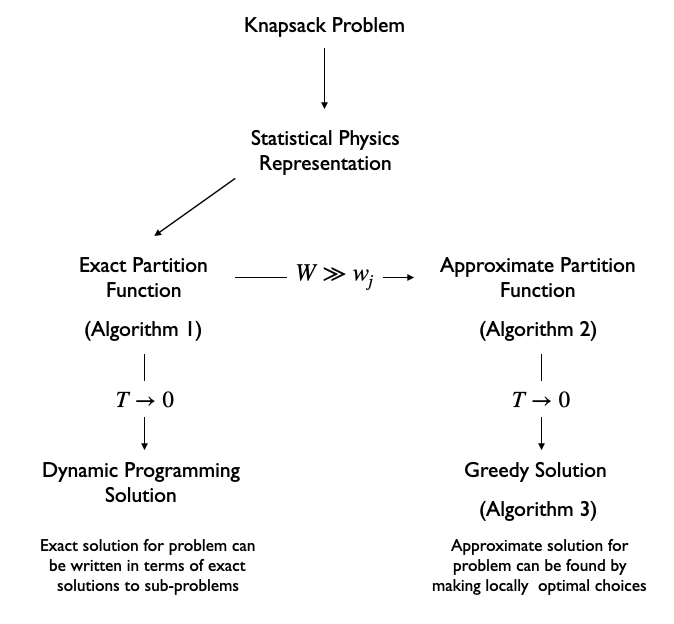
Statistical formalism relates DP and greedy algorithms for KP

Knapsack Instance

The following examples are taken from the example.ipynb file. Run the entire file to reproduce all of the results below.

In the following examples, we will use the item list, weights, values, and weight limits given as follows.

items = (
    ("map", 9, 150), ("compass", 13, 35), ("water", 153, 200), ("sandwich", 50, 160),
    ("glucose", 15, 60), ("tin", 68, 45), ("banana", 27, 60), ("apple", 39, 40),
    ("cheese", 23, 30), ("beer", 52, 10), ("suntan cream", 11, 70), ("camera", 32, 30),
    ("t-shirt", 24, 15), ("trousers", 48, 10), ("umbrella", 73, 40),
    ("waterproof trousers", 42, 70), ("waterproof overclothes", 43, 75),
    ("note-case", 22, 80), ("sunglasses", 7, 20), ("towel", 18, 12),
    ("socks", 4, 50), ("book", 30, 10),
    )

# defining weight and value vectors and weight limit
weight_vec = np.array([item[1] for item in items])
value_vec = np.array([item[2] for item in items])
Wlimit = 400

# defining instance of problem
KP_camping = KnapsackProblem(weights = weight_vec, values = value_vec, limit = Wlimit)

These values are taken from the problem statement in RossettaCode Knapsack: 0-1

Running Large W algorithm

Given weights, values, and a limit, the large W algorithm outputs a list of 1s and 0 corresponding to putting the respective item in the list in the knapsack (output of 1) or leaving said item out (output of 0). From such a list, we can output the final collection of items in the knapsack. To run the algorithm, execute the following code after defining the item list above.

soln = KP_camping.largeW_algorithm()
for k in range(len(soln)):
    if soln[k] == 1:
        print(items[k][0])
        

>>>
map
compass
water
sandwich
glucose
banana
suntan cream
waterproof trousers
waterproof overclothes
note-case
sunglasses
socks

This result reproduces the solution given in RossettaCode Knapsack: 0-1. To apply the algorithm to other knapsack problem instances, replace the values, weights, and limit in the example.ipynb file with the respective quantities for your chosen instance.

Plotting potential function

The potential function for the zero-one knapsack problem is

FN_zero_one = lambda z, weights, values, limit, T: - limit*np.log(z)-np.log(1-z) + np.sum(np.log(1+z**(weights)*np.exp(values/T)))

This function gives a continuous representation of the standard discrete optimization objective. If the function has a local minimum, then the large N algorithm can solve the knapsack problem. This minimum depends on temperature, and as the temperature is lowered the minimum better defines an optimal solution for the knapsack problem. To plot the potential function for the above instance, execute the following code.

KP_camping.plot_potential(T = 1.5)
>>>

Plotting total value as a function of temperature

To plot the calculated total value as a function of temperature, execute the following code

KP_camping.plot_value_vs_temp(temp_low=1.0, temp_high = 60.0)
>>>

This plot uses the nonzero-temperature algorithm to compute the object composition for each temperature between temp_low and temp_high and then computes the total value of that composition. We see that as temperature is lowered, the total value of the collection increases until it presumably has reached its maximum value.

Algorithm comparison plots

In the original paper, we compare the performance of various classic knapsack problem algorithms to the proposed algorithm. The algorithms we compare are

• Brute Force(brute_force): Involves listing all possible combinations of items, computing the total weights and total values of each combination and selecting the combination with the highest value with a weight below the stated limit.

• Dynamical Programming Solution(knapsack_dpV): Standard recursive solution to the problem which involves storing sub-problem solutions in matrix elements

• Fully Polynomial Time Approximate Solution (FPTAS)(fptas): Algorithm that is polynomial time in the number of elements and which has a tunable accuracy

• Greedy Algorithm(greedy): Involves computing the ratio of weights to volumes for each object and filling in the collection until the max weight is reached.

• Simulated Annealing(simannl_knapsack): Involves representing the system computationally as a statistical physics one and then "annealing" the system to low temperatures.

• Exact $Z$ Algorithm:(exact_z_algorithm) Algortihm based on computing the exact partition function recursively for a particular temperature

• Large W Algorithm (T=0):(largeW_algorithm) Algorithm proposed in paper; based on statistical physics representation of the system at $T=0$

• Large W Algorithm (T=0):(largeW_algorithm) Algorithm proposed in paper; on statistical physics representation of the system at $T \neq 0$

A quick comparison of these algorithms for the problem instance shown above is given by the following code.

Assembling needed algorithms and modules

from classic_algos import (brute_force, 
                           knapsack01_dpV, 
                           fptas, 
                           greedy, 
                           simann_knapsack)
from largeN_algo import zero_one_algorithm

from tabulate import tabulate
from collections import defaultdict

import time

Defining dictionary of algorithms and empty dictionary for results

# dictionary of algorithm names and functions
algo_name_dict = {'Brute': KP_camping.brute_force,
                  'DP': KP_camping.knapsack01_dpV,
                  'FPTAS': KP_camping.fptas,
                  'Greedy': KP_camping.greedy,
                  'Annealing': KP_camping.simann_knapsack,
                  'Exact Z': KP_camping.exact_z_algorithm,
                  'Large W (T=0)': KP_camping.largeW_algorithm,
                  'Large W (T/=0)': KP_camping.largeW_algorithm}

# dictionary of algorithm names and results
results_name_dict = defaultdict(lambda: list())

Running algorithm and creating table of results

for name, func in algo_name_dict.items():
    start_clock = time.time()
    if name == 'Large W (T/=0)':
        soln = func(T=1.0)
    else:    
        soln = func()    
    
    # calculating values
    tot_value = str(round(np.dot(value_vec, soln), 0))
    tot_weight = str(round(np.dot(weight_vec, soln), 0))
    time_calc = str(round(time.time()-start_clock, 5)) 
    
    # assembling results
    results_name_dict[name] = [name, tot_value, tot_weight, time_calc]
    
# creating table of results
tabular_results = []
for k, v in results_name_dict.items():
    tabular_results.append(v) 

Printing Table

print(tabulate(tabular_results, ["Algorithm", "Value", "Weight", "Time (sec)"], tablefmt="grid"))
>>>

Stopping annealing because error tolerance was reached
+----------------+---------+-----------+--------------+
| Algorithm      |   Value |   Weight  |   Time (sec) |
+================+=========+===========+==============+
| Brute          |    1030 |       396 |     17.7323  |
+----------------+---------+-----------+--------------+
| DP             |    1030 |       396 |      0.00288 |
+----------------+---------+-----------+--------------+
| FPTAS          |    1030 |       396 |      0.00203 |
+----------------+---------+-----------+--------------+
| Greedy         |    1030 |       396 |      5e-05   |
+----------------+---------+-----------+--------------+
| Annealing      |     945 |       396 |      0.06043 |
+----------------+---------+-----------+--------------+
| Exact Z        |    1030 |       396 |      0.05562 |
+----------------+---------+-----------+--------------+
| Large W (T=0)  |    1030 |       396 |      0.00097 |
+----------------+---------+-----------+--------------+
| Large W (T/=0) |    1030 |       396 |      0.03297 |
+----------------+---------+-----------+--------------+

We see that both large W algorithms yield the correct result, though they are not the fastest algorithms for this instance.

Jupyter notebooks associated with paper

The notebooks that reproduce the figures and tables in the paper are as follows

**

Main Notebooks

• potential_landscape.ipynb: Reproduces Figure 2(a); Runs in < 1 minute
• total_value_vs_temperature.ipynb: Reproduces Figure 2(b); Runs in < 1 minute
• Algorithm Comparison Notebooks
  • algorithm_comparisons_circle.ipynb: Reproduces Figures 3(a), 3(b), and 3(c); Runs in < 20 minutes
  • algorithm_comparisons_spanner.ipynb: Reproduces Figure 3(d), 3(e), and 3(f); Runs in < 20 minutes
  • algorithm_comparisons_profit_ceiling.ipynb: Reproduces Figures 5(a), (b), and (c); Runs in < 20 minutes
  • algorithm_comparisons_multi_strong.ipynb: Reproduces Figures 5(d), (e), and (f); Runs in < 20 minutes
  • *All of the algorithm comparison notebooks include a computation of the the "norm. ratio. diff." for that instance. These computations affirm Eq. (51) in the paper.

Additional Notebooks

• example.ipynb: Not referenced in paper; Example file for the current readme.
• root_finding_algos.ipynb: Not referenced in paper; Notebook for testing various root-finding algorithms
• algorithm_comparisons.ipynb: Not referenced in paper; Applies algorithms to easy instance of the KP
• dynamic_partition_function.ipynb: Not referenced in paper; Shows how to use dynamic programming to compute the partition function and solution of KP for easy instance
• dynamic_partition_comparisons.ipynb: Not referenced in paper; Compares the accuracy and computation time of the exact partition function solution to the KP and the dynamic programing solution to the KP

Acknowledgments

Work completed in Jellyfish Research.