Integrative orthogonal non-negative matrix factorization
An integrative approach to model and predict multiple data sources based on orthogonal matrix factorization. For details of the model, please refer to Stražar M., Žitnik M., Zupan B., Ule. J, Curk. T: Orthogonal matrix factorization enables integrative analysis of multiple RNA binding proteins (to appear).
iONMF can be installed using the pip package manager (may require root privileges):
pip install ionmf
iONMF can then be used within Python scripts. To factorize a NumPy array, type:
    import numpy as np
    from ionmf.factorization.onmf import onmf
    X = np.random.rand(10, 10)
    W, H = onmf(X, k=5, alpha=1.0)
The framework is simple to use within Python scripts. Assume the data is represented as matrices X1, X2, ..., XN - data sources, where rows represent samples and columns represent features. There can be multiple feature matrices as long as they share the same number of rows.
An iONMF model approximates each matrix Xi with a matrix product W Hi, such that
X_1 ~ W H1
X_2 ~ W H2
...
X_N ~ W HN
where W, and H1, H2, ..., HN are non-negative matrices of lower ranks and their matrix product approximates the data sources X1, X2, ... XN.
The coefficient matrix W is common to all data sources and represents clustering of rows, while each basis matrices H1, H2, ..., HN represent clustering of columns. Due to non-negativity constraints, the rows of H can be interpreted as commonly occuring combinations of features.
Such model can be used to provide and interpetation of the dataset (unsupervised learning; clustering of rows and most commonly occuring features) or prediction (supervised learning), where one or more datasource is missing for a set of test samples, provided at least one Xi is available.
The data is assumed to be stored in one or more Numpy arrays (numpy.ndarray) and contain only non-negative values.
The dataset is then stored as a dictionary:
dataset = {
  "data_source_1": X1,
  "data_source_2": X2,
  "data_source_3": X3,
  # etc.
}
where the keys are data source names and X1, X2, X3 represent matrices (Numpy arrays having the same number of rows.)
The model is initizalized as a class as follows
from ionmf.factorization.model import iONMF
model = iONMF(rank=5, max_iter=100, alpha=1.0)
where rank is the maximum rank of the low-rank approximation, max_iter the number of iterations during optimization and alpha the orthogonality regularization. Higher alpha yields more distinct (orthogonal) basis vectors.
Having prepared the dataset, the model is trained as follows:
model.fit(dataset)
THe low-rank approximations can be accessed e.g.
model.basis_["data_source_1"]  # Get the basis (H) matrix for data_source_1
model.coef_                    # Get the coefficient (W) matrix
Next, suppose we have a another set of samples, where one or more data sources are missing.
testset = {
  "data_source_1": Y1,
  "data_source_3": Y3,
}
In this example, the data_source_2 is missing. Again, Y1, Y3 must share the same number of rows. Having trained a model on the previous (training) dataset,
the missing data sources can be filled in.
results = model.predict(testset)
The result is a dictionary results that contains approximations to all data sources that were missing from testset, in this case, data_source_2.
Y2 = results["data_source_2"]
Prepared practical examples for usage of the model are available.
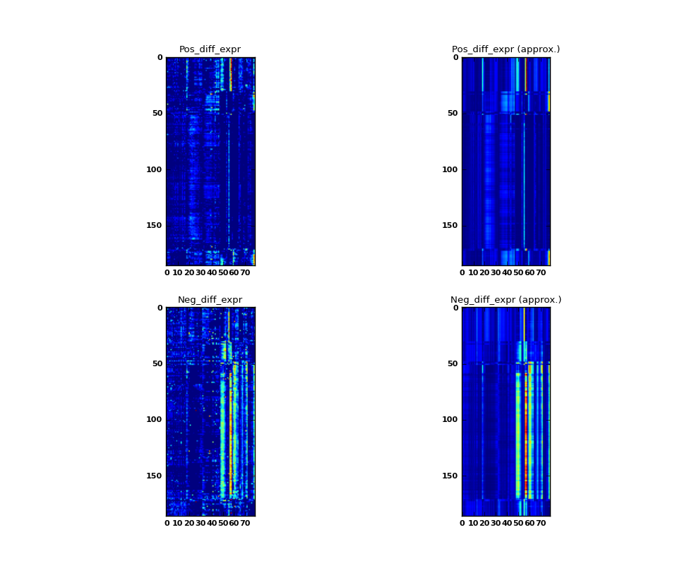
See ionmf.example.yeast_rpr.py A simple example of running iONMF on a differential gene expression dataset. The dataset contains 186 samples and 79 genes, divided into 3 classes.
Some values in the matrix X contain negative values. The following trick is used. The number of columns is doubled to form the matrices Xp, Xn each of size (186 rows, 79 columns). All positive values are stored in Xp, while absolute values of negative cells are stored in Xn.
Additional three 186 x 1 matrices are stored to represent the three classes (value 1 if the sample i belongs to the class).
In this demonstrative example, the model is trained on the whole dataset. In the test phase, the datasources representing classes are removed from the model. After prediction, each sample is assigne to class 0, 1, or 2 depending on maximum value in approximated columns class_0, class_1, class_2. The training accuracy is measured as the fraction of correctly classified examples.
Each matrix X is plotted along with the approximation W H. Increasing the maximum model rank would yield more accurate approximations.
The details of each step is explained in the comments.
An application is presented on modeling protein-RNA interaction data as presented in the article above. Currently, 31 CLIP datasets are available corresponding to the numbering adopted in the article. Each training and test set contains 20% positive (cross-linked positions) and additional data sources: RNA k-mers, RNA structure (as predicted with RNAfold), Region types (genomic annotation), GeneOntology terms and Co-bining (CLIP experiments on other proteins that are not technical or biological replicates).
The master branch include only one training/test sample of positions of size 5000 per protein.
Larger datasets with 30000 positions as well as more training/test splits are available at
branch master_full. For more details on the format of data, see /datasets/clip/README.html.
Characteristic data-source featue values, presented in the article Suplementary Section 7 are
available within branch master_full at /features
An example is run as follows
cd ionmf/examples/
export PYTHONPATH="../.."
python clip.py  27_ICLIP_TDP43_hg19
where the argument is one of the datasets within the collection:
datasets/
  clip/
    1_PARCLIP_AGO1234_hg19
    2_PARCLIP_AGO2MNASE_hg19
    3_HITSCLIP_Ago2_binding_clusters
    4_HITSCLIP_Ago2_binding_clusters_2
    5_CLIPSEQ_AGO2_hg19
    6_CLIP-seq-eIF4AIII_1
    7_CLIP-seq-eIF4AIII_2
    8_PARCLIP_ELAVL1_hg19
    9_PARCLIP_ELAVL1MNASE_hg19
    10_PARCLIP_ELAVL1A_hg19
    11_CLIPSEQ_ELAVL1_hg19
    12_PARCLIP_EWSR1_hg19
    13_PARCLIP_FUS_hg19
    14_PARCLIP_FUS_mut_hg19
    15_PARCLIP_IGF2BP123_hg19
    16_ICLIP_hnRNPC_Hela_iCLIP_all_clusters
    17_ICLIP_HNRNPC_hg19
    18_ICLIP_hnRNPL_Hela_group_3975_all-hnRNPL-Hela-hg19_sum_G_hg19--ensembl59_from_2337-2339-741_bedGraph-cDNA-hits-in-genome
    19_ICLIP_hnRNPL_U266_group_3986_all-hnRNPL-U266-hg19_sum_G_hg19--ensembl59_from_2485_bedGraph-cDNA-hits-in-genome
    20_ICLIP_hnRNPlike_U266_group_4000_all-hnRNPLlike-U266-hg19_sum_G_hg19--ensembl59_from_2342-2486_bedGraph-cDNA-hits-in-genome
    21_PARCLIP_MOV10_Sievers_hg19
    22_ICLIP_NSUN2_293_group_4007_all-NSUN2-293-hg19_sum_G_hg19--ensembl59_from_3137-3202_bedGraph-cDNA-hits-in-genome
    23_PARCLIP_PUM2_hg19
    24_PARCLIP_QKI_hg19
    25_CLIPSEQ_SFRS1_hg19
    26_PARCLIP_TAF15_hg19
    27_ICLIP_TDP43_hg19
    28_ICLIP_TIA1_hg19
    29_ICLIP_TIAL1_hg19
    30_ICLIP_U2AF65_Hela_iCLIP_ctrl_all_clusters
    31_ICLIP_U2AF65_Hela_iCLIP_ctrl+kd_all_clusters
A desired subset of data sources is seleted via the method
def load_data(path,
    kmer    = True,   # RNA k-mers
    rg      = True,   # Region Type
    clip    = True,   # Experiments (cobinding)
    rna     = True,   # RNAfold structure prediction
    go      = True,   # Gene Ontology terms
    )
A run including all data sources required 12 GB of RAM and completes in 21 minutes on a 2GHz CPU. Support for sparse matrices is under construction.
A single training / prediction run is perfomed.
The positions in the test samples are sampled from genes that do not overlap with training genes. The exact location of the positions can be examined in the corresponding .bedGraph text file, e.g.: datasets/clip/27_ICLIP_TDP43_hg19/2000/training_sample_0/positions.bedGraph.gz
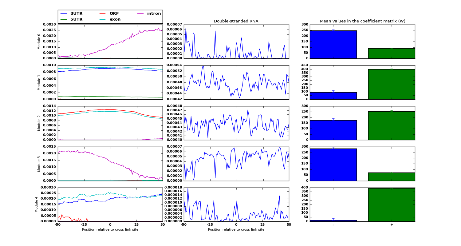
Examples of low-dimensional modules for the data sources RNA structure and region types, along with an estimate of each module belongin to either positive/negative examples is shown:
The details of each step is explained in the comments within the script.