The emergence of Peer-to-Peer (P2P) lending has revolutionized the loan market by directly connecting borrowers with investors. A pivotal aspect of this market is the determination of appropriate loan rates. Loan rates are crucial as they reflect the risk associated with lending money. It also significantly influences the borrower’s ability to repay the loan and the investor’s return on investment. If the loan rate is too high, the debtors might default and fail to meet the repayment deadline. The creditor cannot get a satisfactory investment return if the loan rate is too low.
Our primary research objective is to use the LendingClub dataset to develop a predictive model for loan rates. This model aims to estimate the interest rate assigned to a loan based on various predictors. These predictors could include borrower-specific information such as credit score, income level, employment history, and loan-specific details like loan amount and loan purpose.

Remark: This is a Final Project for the course QTM 347 "Machine Learning" offered by Emory University. The contributors to this project are Ruichen Ni, Alex Ng, Haoyang Cui, and Mo Zhou. The instructor of this project is Dr. Ruoxuan Xiong at the Quantitative Sciences Department of Emory University.
| Variable Name | Description | Data Type |
|---|---|---|
| loan_amnt | The total amount of the loan | Numeric |
| loan_term | The term of the loan (in months) | Numeric |
| emp_length | Employment length (in years) | Categorical |
| home_ownership | The home ownership status | Categorical |
| income_source_verified | Indicator if income source was verified | Binary |
| income_verified | Indicator if income was verified | Binary |
| income_thou | Income in thousands | Numeric |
| debt_income | Debt-to-income ratio | Numeric |
| delinq_2yrs | The number of 30+ days past-due incidences of delinquency in the borrower's credit file for the past 2 years | Numeric |
| credit_history_length | Length of the borrower's credit history | Numeric |
| FICO | FICO credit score | Numeric |
| open_acc | Number of open credit lines | Numeric |
| derogatory_recs | Number of derogatory records | Numeric |
| revol_balance | Total credit revolving balance | Numeric |
| revol_util | The amount of credit the borrower is using relative to all available revolving credit. | Numeric |
| loan_rate | Interest rate of the loan (Our Research target) | Numeric |
The traditional method of determining loan rates often relies on somewhat arbitrary factors, and it involves a lengthy process that necessitates the involvement of trained staff. While potentially suitable for conventional financial institutions such as commercial banks where thoroughness is prioritized over speed, this approach may not align well with the needs of Peer-to-Peer (P2P) lending platforms that value prompt service and efficiency. In the context of P2P platforms, which operate in a more dynamic and fast-paced environment, the traditional loan rate determination process can be seen as cumbersome and time-consuming.
To address this challenge, integrating a machine-learning algorithm could significantly enhance the efficiency of the lending process for these platforms. Machine learning offers the ability to quickly, accurately, and objectively analyze vast amounts of data. By automating the analysis of borrower data, these algorithms can provide rapid and more objective assessments of credit risk, leading to quicker loan rate determinations. This streamlines the process and potentially reduces the likelihood of human error or bias in setting loan rates.
This approach has significant benefits compared to traditional methods. It can rapidly process large volumes of data, providing loan rates much quicker than manual methods. It could be vital in P2P platforms, where both lenders and borrowers value efficiency and timeliness.
From the data description section, we can see that there are two categorical variables, "Home" and "Employment length." To incorporate them into our regression model, we transform them into dummies. The 'Home' variable has three possible values: 'MORTGAGE,' 'OWN,' and 'RENT.' To avoid multicollinearity, we only keep 'MORTGAGE' and 'RENT" in our dataset. Similarly, for 'Employment length,' we dropped 'emp_length_<1 year' for the same reason.
Note: Related codes can be found in the in ‘Data Cleaning’ file in the "Data description" folder of this project.
To start with, we explored our data with several visualizations:
Click to expand
1.1 Correlation Heatmap of the Variables.
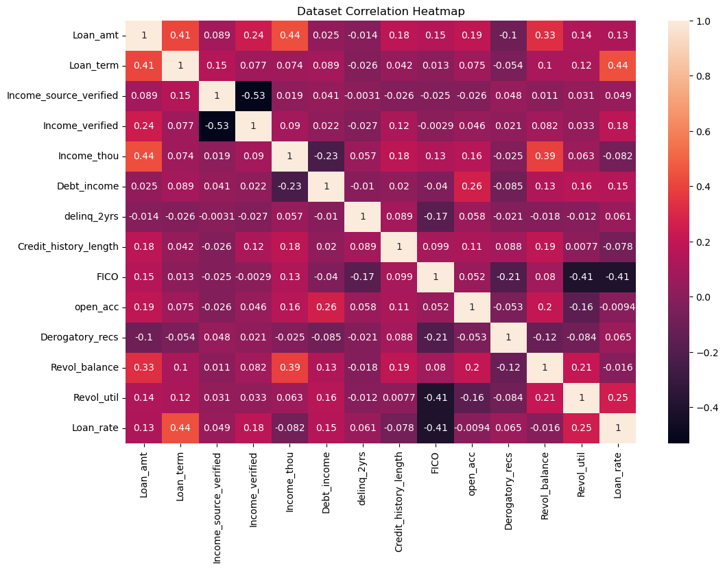
From the map, we can observe that:
-
Loan_term appears to have a moderate positive correlation with loan_rate, indicated by a coefficient value of 0.45. This suggests that as the term of the loan increases, the loan rate tends to be higher.
-
FICO score shows a negative correlation with loan_rate, with a coefficient of -0.41. This indicates that higher FICO scores, which suggest better creditworthiness, are associated with lower loan rates.
-
Revol_util (revolving line utilization rate) has a positive correlation with loan_rate at a value of 0.25, suggesting that higher utilization rates of available credit may lead to higher loan rates.
-
Debt_income (debt-to-income ratio) and Income_thou (income in thousands) have weaker positive correlations with loan_rate, with coefficients of 0.15 and 0.13, respectively, implying a less pronounced relationship with the loan rate.
Other variables, such as Loan_amt (loan amount), Income_source_verified, and Open_acc (number of open credit lines), show very weak correlations with loan_rate, as indicated by coefficients close to 0.
1.2 Frequency Plot of FICO Score
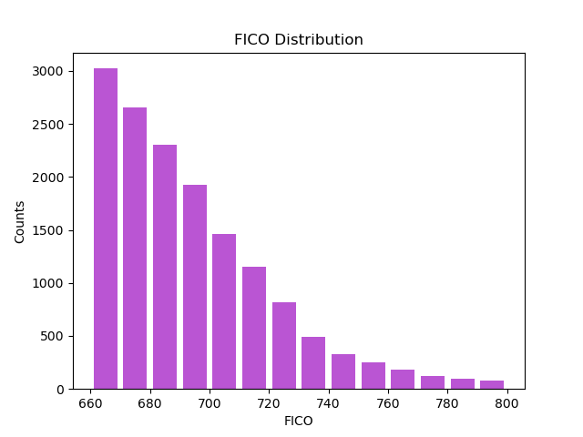
The minimum FICO score for applicants who are granted the loans is 662, showing that there is a minimum FICO requirement for applicants to receive the loans.
The highest frequency occurs in the lower FICO score intervals, starting with the 660 range. This suggests that a larger number of individuals in the dataset have lower FICO scores.
As the FICO score increases, the frequency of individuals within those intervals decreases. This implies that fewer individuals have higher FICO scores.
The distribution appears to be right-skewed, meaning there is a longer tail towards the higher end of the FICO score spectrum. This skewness indicates that while most of the scores are concentrated on the lower end, there are still some individuals with very high credit scores, but they are less common.
1.3 Frequency Plot of Loan Amount
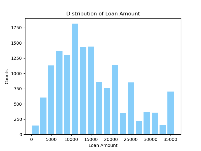
There is a relatively high frequency of loans in the lower loan amount ranges, starting from 0 up to around 15000. This suggests that most individuals in the dataset are taking out smaller loans.
The highest frequency of loans seems to occur in the 10000 to 15000 range, indicating that this loan amount range is the most common among the dataset's individuals.
As the loan amount increases beyond the peak range (15000), the frequency of loans gradually decreases, which means that larger loans are less common in this dataset.
The distribution may have multiple modes (peaks), as there seem to be several intervals with high frequencies, which suggests that certain loan amounts are particularly common, potentially due to common financing needs or lending products offered.
Overall, the distribution of loan amounts in this dataset is multimodal and shows that smaller loans are more frequently taken out than larger ones, with particular loan amounts appearing to be more popular than others.
1.4 Frequency Plot of Log Income
Because the data has a long-tail effect, we log-transform it.
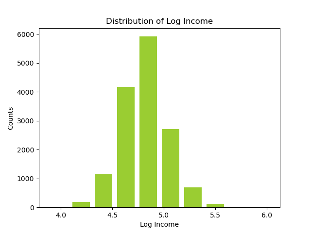
A peak in the distribution, which seems to occur around the 4.5 to 5.0 log income value, indicates that the majority of incomes in the dataset cluster around 31622 (
The bars at the lower and higher ends of the spectrum have lower counts, suggesting fewer individuals with very low or very high incomes, relative to the central peak.
The shape of the distribution could be somewhat bell-shaped with a peak in the middle, indicating that the underlying income distribution, before the log transformation, is right-skewed, which is typical for income data where a large number of people earn moderate incomes and fewer people earn extremely high incomes.
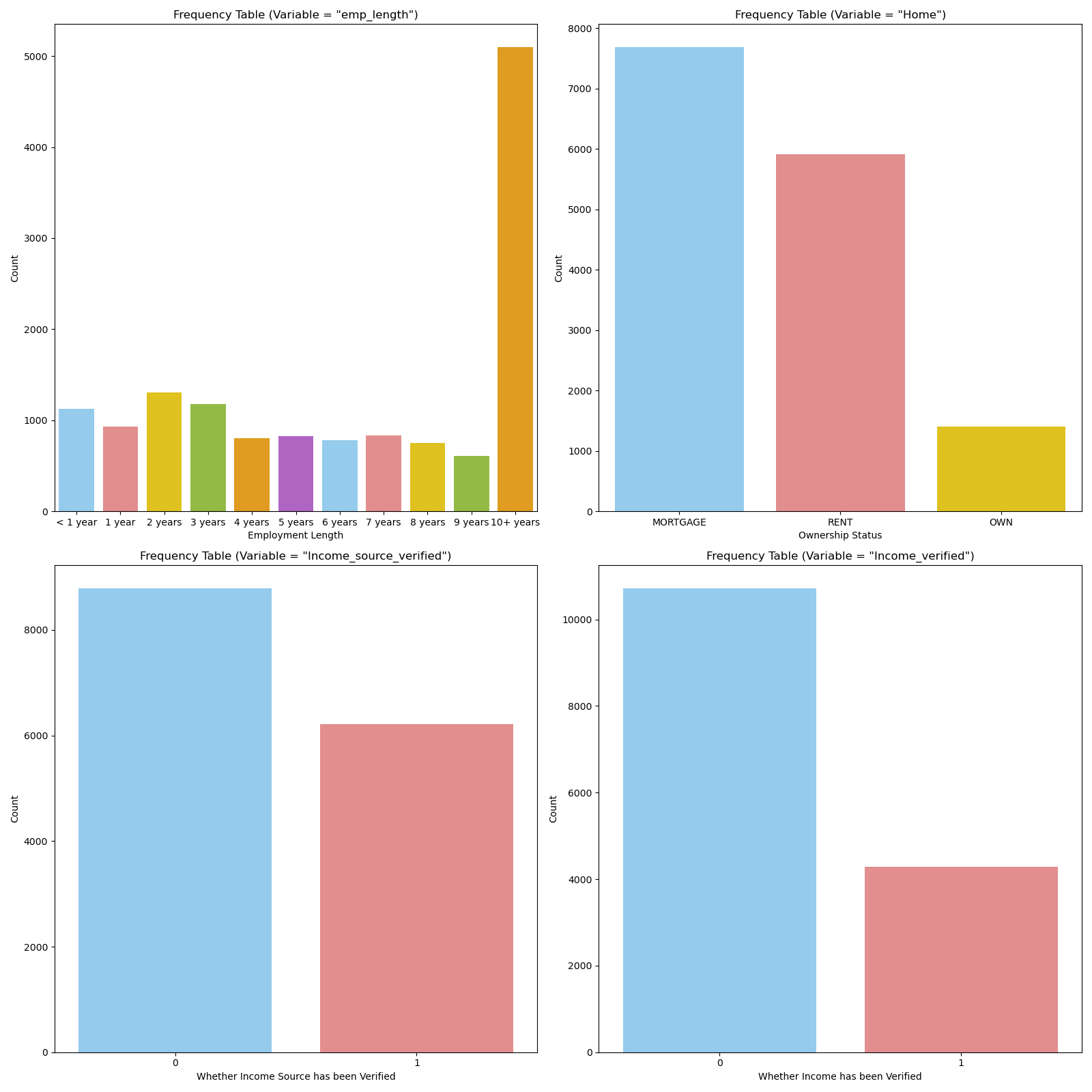
1.5 Frequency Table of Categorical Variables
-
Empolyment Length: Generally, the number of loan applicants shows a decreasing pattern as employment length increases. However, the data does not distinguish employment length after 10 years, so we can observe there is a large amount of applicants with 10+ years working experience.
-
Home Ownership Status: The home ownership status graph might show a higher frequency for "MORTGAGE" and "RENT," as these are common living situations. The frequency for "OWN" might be lower, reflecting the smaller proportion of individuals who own their homes outright without a mortgage.
-
Income Source Verification and Income Verification: Those two graphs show that most applicants do not have their income source and income verified.
1.6 Frequency Table of Loan Rate
IMAGE HERE Description here
Note: Related codes can be found in the ‘visual’ file in the "Data description" folder of this project.
All the codes in this project are executed under a Python 3.8+ environment. Our computing environment is a MacBook Pro 2021 with an M1 Max Chip and 32 GB of memory. Even though we are confident that less sophisticated computer systems could also run these codes, we expect them to take more than 30 minutes to go through all the codes.
Parametric models are the simplest and most intuitive way of modeling the loan rate. However, since some of the predictor variables show small correlations with the response, incorporating those predictors in our model will be problematic for an accurate, consistent prediction. Therefore, we introduce some methods for variable selection and dimensional reduction.
Click to expand
Forward Selection is a stepwise approach in model building where predictors are added one at a time to a regression model, starting with the variable most strongly associated with the response variable. At each step, the variable that provides the greatest additional improvement to the model fit is included until no more significant variables are found, or a specified criterion is met. For our dataset with many predictors, this method could be computationally more convenient than traditional subset selection methods.
Backward Selection is also a stepwise approach in modeling where all potential predictors are initially included, and then the least significant variables are removed one by one. This process continues until only variables that contribute significantly to the model's predictive power remain, ensuring a more parsimonious and potentially more interpretable model.
PCR is useful for variable selection as it reduces the dimensionality of the data by selecting a few principal components, which are linear combinations of the original variables, thus simplifying the model without significantly losing information. It combines Principal Component Analysis (PCA) and regression and is useful for handling multicollinearity in regression models.
Like Principal Component Regression (PCR), PLS reduces the dimensionality of data but focuses more on predicting a dependent variable by finding the multidimensional direction in the space of the independent variables that explains the maximum multidimensional variance of the dependent variable. It not only reduces the number of variables but also maintains the ones most relevant for predicting the dependent variable.
To reduce the probability of overfitting, we introduce regularization methods:
Click to expand
Ridge regression is a technique used to analyze multiple regression data that suffer from overfitting. It reduces the standard error by adding a bias parameter in the estimates of the regression and shrinking large parameters to avoid overfitting issues.
Lasso regression is a type of linear regression that uses shrinkage: it applies a penalty to the absolute size of the regression coefficients. This method not only helps in variable selection by shrinking less important coefficients to zero but also improves the prediction accuracy and interpretability of the statistical model.
Elastic Net is a regularization technique in linear regression that combines the penalties of both Ridge and Lasso regression methods, helping to overcome the limitations of each when dealing with highly correlated variables or when selecting features. Its primary advantage over Ridge and Lasso is its ability to select groups of correlated variables, which Ridge can't do, and to maintain a more stable and accurate model than Lasso when dealing with numerous features or highly correlated predictors.
The models listed so far, though variegated in their specific implementation, only capture linear relations between predictors and the response variable. However, we are not confident that the predictor variables have linear relationships with the response variable. If we want to catch non-linear relationship between those variables, we should also include some non-parametric methods:
Click to expand
The KNN method predicts the outcome for a new data point by analyzing the K closest data points (neighbors) from the training set. It's based on the principle that similar data points tend to have similar outcomes, making it a popular choice for its ease of understanding and implementation, especially in scenarios where relationships between variables are complex or unknown.
A Decision Tree is a flowchart-like tree structure where each internal node represents a test on an attribute, each branch represents the outcome of the test, and each leaf node represents a class label or regression value used for making predictions based on simple decision rules. Random Forests, on the other hand, is an ensemble learning method that operates by constructing multiple decision trees during training and outputting the class that is the mean prediction (regression) of the individual trees, offering improved accuracy and robustness over a single decision tree. Bagging is similar to Random Forests in that both methods use an ensemble of decision trees and bootstrap sampling, but Random Forest introduces additional randomness by selecting random subsets of features for splitting each node, whereas bagging uses all features.
Gradient Boosting is a technique that builds models in a stage-wise fashion, similar to the rationale of PLS and PCR. It combines the predictions of multiple decision trees to create a strong predictor, optimizing a loss function by iteratively adding new models that correct the errors of the previous ones, making it highly effective for complex datasets with non-linear relationships.
In the following few paragraphs, we will describe the main results and thought processes associated with each one of these models.
Here are the results concerning the parametric models we implemented:
Click to expand
To start with, we performed the forward and backward variable selection based on the R-squared of the fitted linear regression. We graphed RSS, Adjusted R-squared, AIC, and BIC with respect to the number of predictors selected. The results for forward and backward selections are very similar:

The red dot in each graph indicates the number of predictors that generate the lowest training error based on the given criterion. As a result, we would follow BIC, which gives us a simpler model that uses only selected 14 predictors. In doing so, we can prevent overfitting. The models generated by forward selection and backward selection based on BIC are exactly the same, which is summarized below:
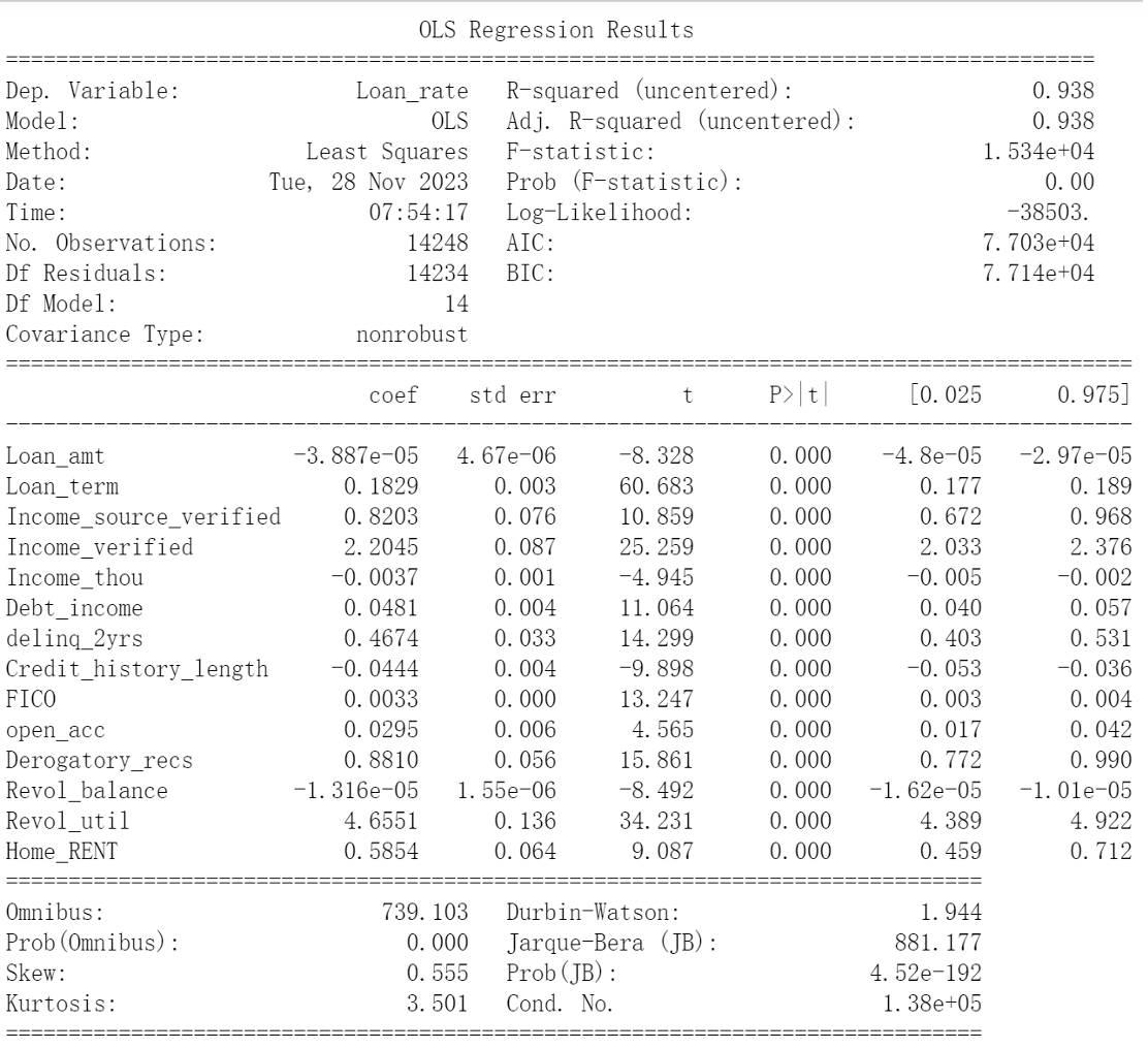
Then, we refitted the linear regression model with the 14 best predictors we selected and used it to predict the testing set. The resulting test MSE is 10.945027615948739.
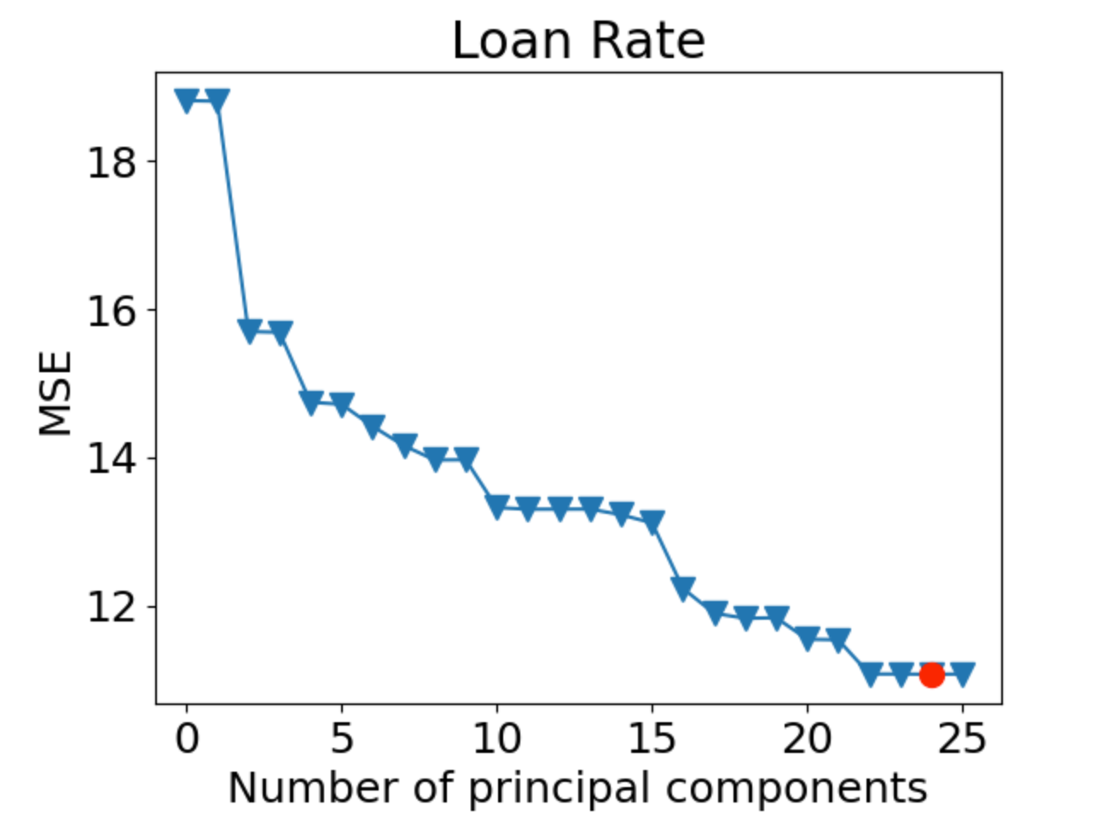
Next, we ran the Principal Component Regression (PCR) and Partial Least Square Regression (PLS), both with the number of principal components (n) selected from 10-fold cross-validation. We graph the cross-validation MSE with respect to ‘n’.
For PCR:
For PLS:
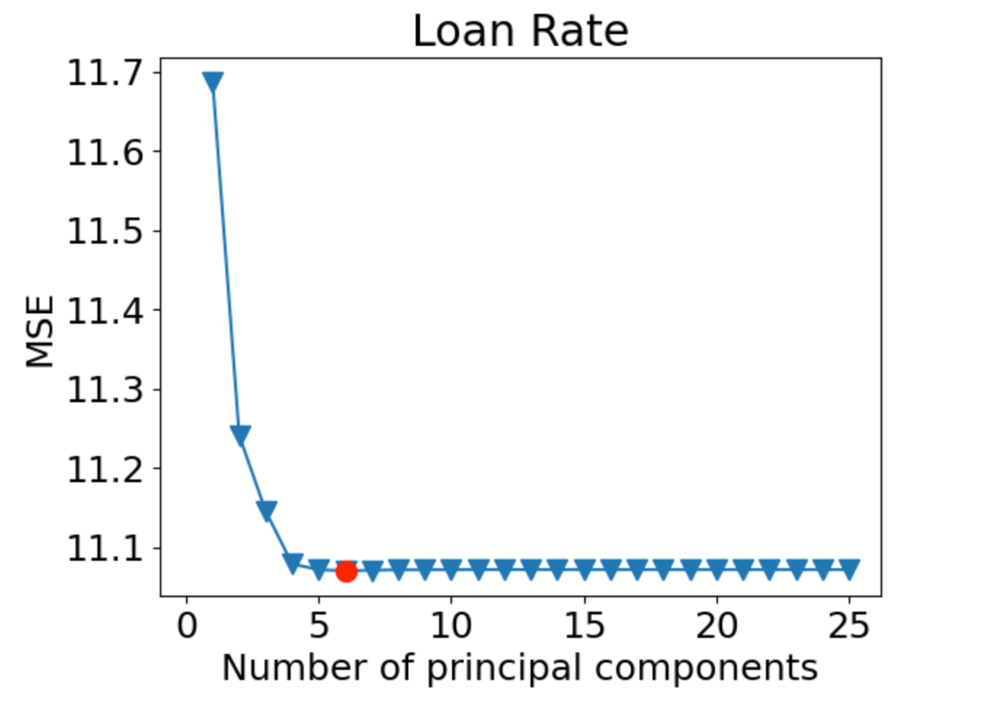
Based on the two figures above, we can see that the optimal number of principal components for PCR is n=24, and the optimal number of principal components for PLS is n=6. We refitted both models with the selected number of components ‘n’ and used them to predict on the testing set. The resulting test MSE for PCR is 10.69176181204259, and the resulting test MSE for PLS is 10.693106578498861.
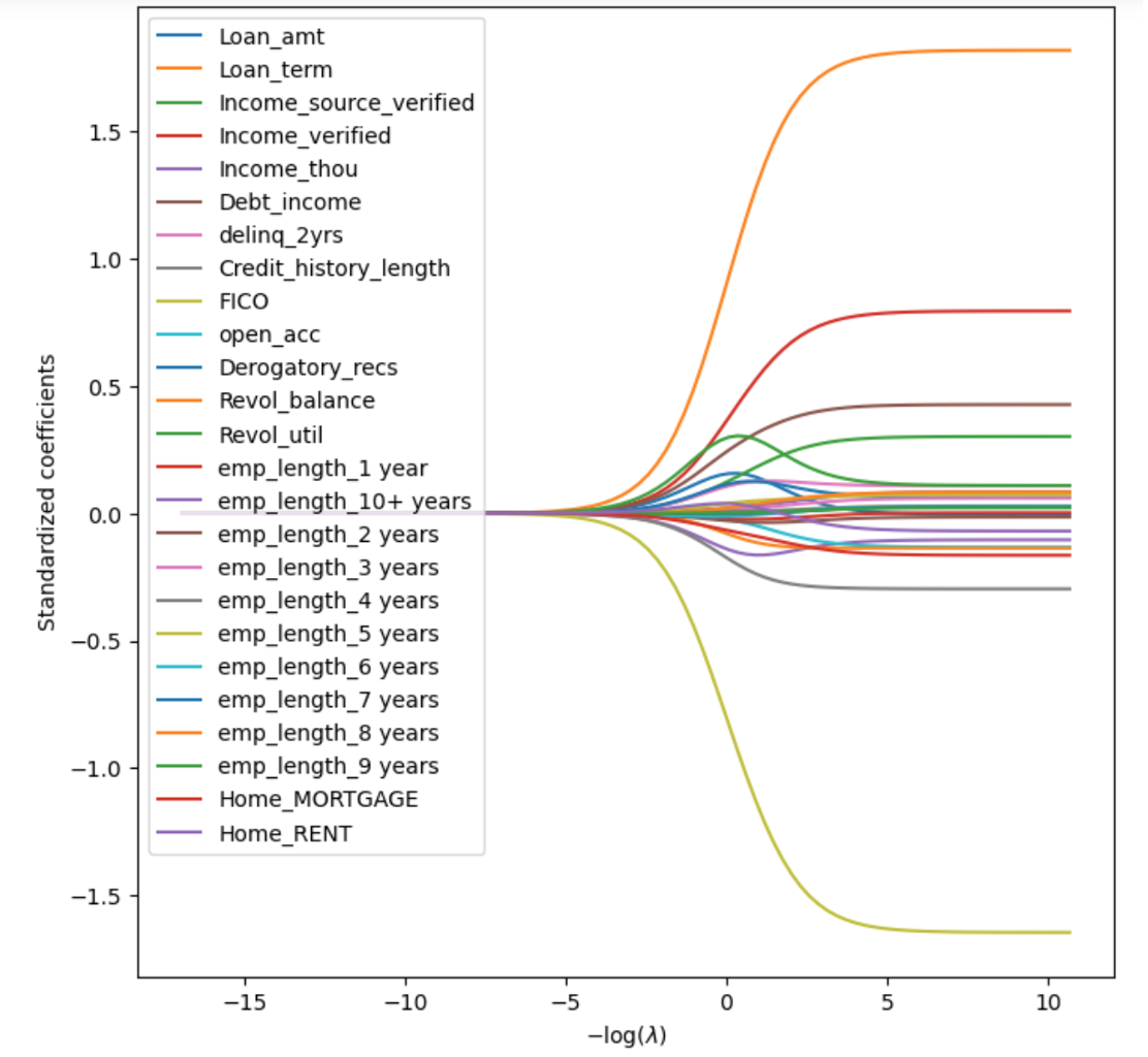
Then, we run the Ridge Regression and Lasso Regression. To start with, we graph the change in the standardized regression coefficients with respect to -log(λ) for both models, where λ is the tunning hyper-parameter.
For Ridge Regression:
For Lasso Regression:
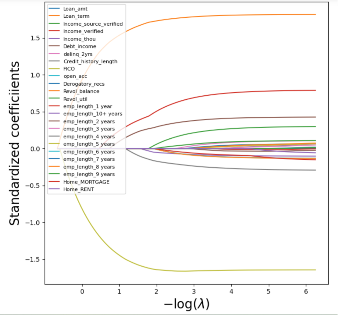
As we can see, as λ increases (-log(λ) decreases), the regression coefficients in both Ridge and Lasso Regression decrease. Lasso Regression can shrink the coefficients to 0, while Ridge Regression can shrink the coefficients to a small number, but not to 0.
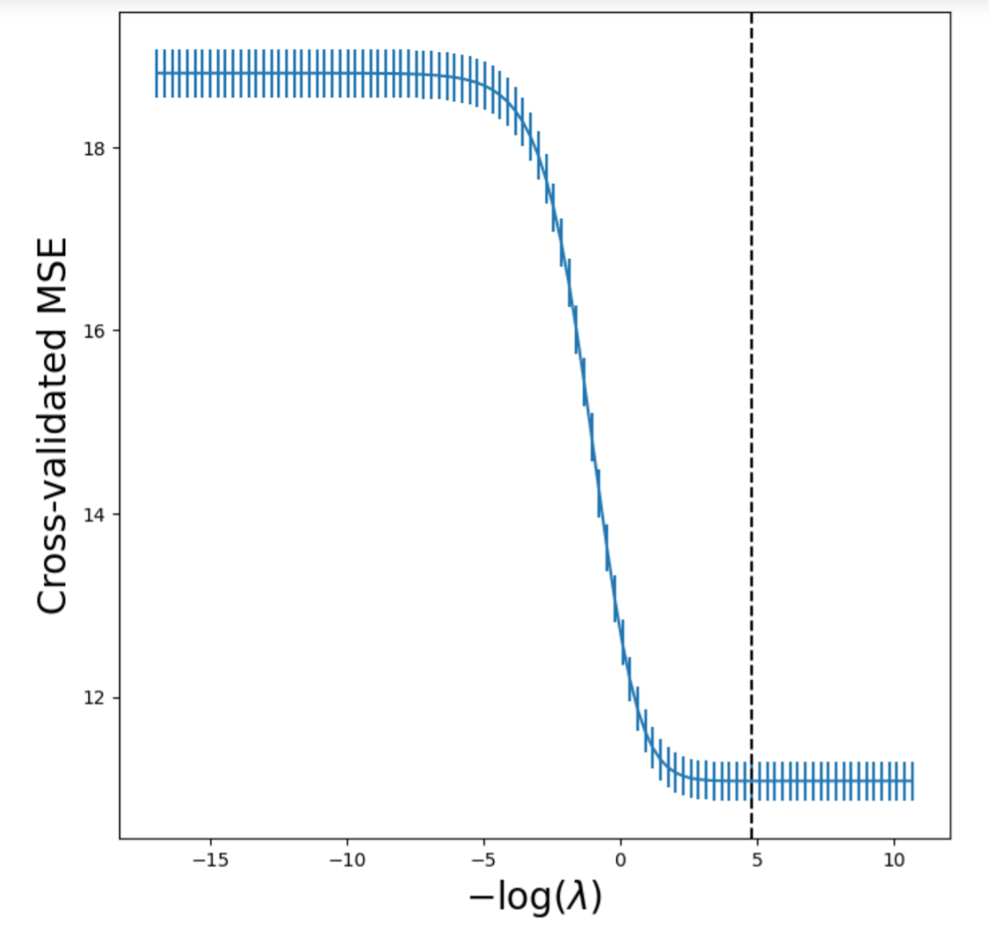
Next, we selected the tunning hyper-parameter λ in both models with 5-fold cross-validation. The validation MSE is graphed with respect to -log(λ):
For Ridge Regression:
For Lasso Regression:
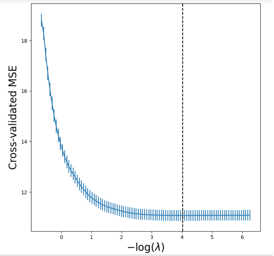
The optimal λ for Ridge Regression chosen by cross-validation is λ = 0.0080967435201. The optimal λ for Lasso Regression chosen by cross-validation is λ = 0.0179450167158. We refitted both models with the optimal λ and used them to predict the testing set. The resulting test MSE for Ridge Regression is 10.699063670936091, and the resulting test MSE for Lasso Regression is 10.691531404491021.
A similar approach also works for the Elastic Net Regression. We first found the tunning parameters λ and α using cross-validation, then refitted the model with the optimal λ and α, and finally used the model to predict on the testing set. The resulting parameters found using 5-fold cross-validation are λ= 0.01993890746208 and α=0.9 (α is selected from {0.1,0.2 ..., 0.9}). The test MSE of the fitted Elastic Net Regression model using the optimal λ and α is 10.6917359885709.
Note: Related codes can be found in the ‘Variable Selection, PCR & PLS’ file and the ‘Regularization (with Lasso & Ridge & Elastic Net)’ file in the "Parametric Model" folder of this project.
Here are the results concerning the parametric models we implemented:
Click to expand
The first nonparametric model we implemented is KNN regression. We first standardized the training and testing feature sets, and then chose the optimal number of neighbor ‘N’ (ranging from 5 to 200) through 5-fold cross-validation. In our case, N=19 was chosen. Then, we refitted the model using N=19 and predicted on the testing set. The resulting test MSE for KNN Regression is 11.4571313245.
Next, we proceeded to implement the regression tree model. To start with, we do not place any restrictions on the tree, and fit the tree on the training data. Following is the plot for the tree:

The resulting tree looks terrible as it keeps growing and ends up having many layers. This tree will undoubtedly overfit our data. The resulting test MSE based on this regression tree is 12.633312900342.
To prevent overfitting, we performed pruning on our tree. We started with using 5-fold cross-validation to find the optimal tuning parameter α. The optimal α we found is α= 0.0288556240014. Then we refitted the regression tree using the optimal tunning parameter α and predicted it on the testing set. The resulting test MSE becomes 11.24517409887, which is smaller than before. Following is the tree after pruning, which has fewer layers:

Then, we implemented Bagging and Random Forest. Notice that Bagging is simply a Random Forest that takes all features into consideration when constructing each tree. For both Bagging and Random Forest, we chose the number of trees ‘n_estimators’ from {100, 200, 300, 400} and {100, 200, 300, 400, 500} respectively through 5-fold cross-validation. We only included a limited number of values for ‘n_estimators’ because the runtime for a larger number of n_estimators is extremely long. Also, for Random Forest, we followed the convention to take the square root of the number of available features as the parameter ‘max_feature’. Since we have 25 features in total, we chose max_feature=5, which means our Random Forest model will consider 5 features when constructing each tree.
The parameter ‘n_estimators’ chosen by cross-validation for Bagging and Random Forest are n_estimators = 400 and n_estimators = 500 respectively. After refitting Bagging and Random Forest with the selected values of n_estimators and predicting on the testing set, the resulting test MSE we got for Bagging and Random Forest are 9.9029367190 and 9.61915126284 respectively.
We can also obtain the 10 most important features based on the Random Forest we built:
IMAGE HERE
Eventually, we implemented the Gradient Boosting Regression (GBR). For GBR, we started by choosing the parameter ‘max_depth’, the maximum depth allowed for the regression tree, through 5-fold cross-validation from integers ranging from 3 to 11. While doing the cross-validation, we selected a high learning rate (0.1) to save some time since there are many features and samples. Also, we selected a larger number for ‘n_estimators’ (‘n_estimators’ =1000) because Gradient Boosting is relatively robust to over-fitting. Larger values for ‘n_estimators’ correspond to lower test MSE as demonstrated by our figure:

Based on the cross-validation, the optimal value of ‘max_depth’ is 5. Then, we refitted the GBR model using max_depth=5. Also, we lowered the learning rate to 0.01 when refitting, since a smaller learning rate will likely generate more accurate model predictions in our case. After refitting the GBR model and predicting the testing set, we obtained a test MSE of 9.4366903363. Because of the large sample size and a large number of features, it takes an extended amount of time to perform cross-validation and find the optimal configuration for parameters such as max depth and sample split. However, the boosted tree gave us the best model among other choices with the lowest test MSE.
We can also obtain the 10 most important features based on the GBR model we built:
IMAGE HERE
Note: Related codes can be found in the’ Non-parametric Model (KNN & Decision Tree)’ file in the "Non-Parametric" folder of this project.
Following is a table of summary for the test MSE, test RMSE, and parameters of each model:
Update the table
| Model | Test MSE | Parameters |
|---|---|---|
| Multiple Linear Regression with Forward Variable Selection | 10.9450 | Number of predictors n=14, chosen based on BIC |
| Linear Regression Based on PCR | 10.6918 | Number of principal components n=24, chosen by cross-validation |
| Linear Regression Based on PLS | 10.6931 | Number of principal components n=6, chosen by cross-validation |
| Ridge Regression | 10.6991 | Value of tunning hyper-parameter λ=0.0081, chosen by cross-validation |
| Lasso Regression | 10.6915 | Value of tunning hyper-parameter λ= 0.0179, chosen by cross-validation |
| Elastic Net Regression | 10.6917 | Value of tunning hyper-parameters λ= 0.0199 and α=0.9, chosen by cross-validation |
| KNN Regression | 11.4571 | number of neighbors N=148, chosen by cross-validation |
| Regression Tree (with pruning) | 11.2452 | Tunning parameter α=0.0288, chosen by cross-validation |
| Bagging | 9.9029 | Number of Trees n_estimators=400, chosen by cross-validation. |
| Random Forest | 9.6192 | Number of Trees n_estimators=500, chosen by cross-validation |
| Gradient Boost | 9.4367 | Maximum depth max_depth=5, chosen by cross-validation. Fixed n_estimators=1000 and learning_rate=0.01 |
Having provided all the model results we gained, we proceed to make some diagnosis and reflections upon our results. The reflections will be divided into two parts: overall diagnosis and model-specific diagnosis.
Overall, the test MSE generated by different models fluctuate between 9 and 12. Also, the test root mean square error (RMSE) generated by different models flunctuate between 3.07 and 3.38. Given that the loan rate (our dependent variable) is provided in percentage scale (e.g. 15 in the data represents a loan rate of 15%) ranging from 6.03 to 26.06 with a mean of 13.83, the overall test RMSE generated by our models is reasonably large. RMSE has the same scale as our target variable (loan rate), so an RMSE of 3.07 given by the GBR model, for instance, would imply that the model produced an average prediction error of 3.07% in comparison with the actual loan rates (with extra weight added to larger prediction errors).
Following are a series of general diagnosis concerning our data, models, and approaches:
Click to expand
- The data itself might be very noisy, since the loan rates for individuals provided in the data were determined subjectively by Lending Club.
- The incomes and income sources of more than half of the individuals in the data have not been verified, so the income data might contain errors. This might greatly influence the accuracy of our predictions since income is an important factor in determining the loan rates.
- We did not take any actions to control for problems associated with multicollinearity, endogeneity, or heteroskedasticity when we ran models based on linear regression.
- There might have been other important variables highly correlated with the loan rate received by an individual that are omitted.
A potential way to improve the overall performance of the models is to change the target variable from the loan rate to the probability of default, and then find a function that maps an individual’s probability of default and the loss given default to the ultimate loan rate. The logistic behind such an improvement is that the data for loan rates in our data has been determined subjectively by lending club, therefore using them directly for training and testing our models might introduce too much noise. The probability of default, however, is much more objective in nature since whether a given individual default is an outcome that can be directly observed. Therefore, the probability of default might be a more suitable target variable for our experiment, though the function that maps an individual’s probability of default and the loss given default to the loan rate can be very difficult to find.
For some of the models, we provide a brief diagnosis and some suggestions for improvements if applicable.
Click to expand
Based on the results, the test MSE generated by PLS is slightly larger than the test MSE generated by PCR. This is very unexpected. Since PCR derives the components only based on predictors and ignores the target variable in our training set, we naturally expect it to perform worse than PLS. The fact that PLS performs worse than PCR in our case suggests that the overfitting problem is serious for the PLS. To prevent overfitting problem, further regularization techniques maybe needed.
KNN produced a test MSE of 11.457, which is the highest among the test MSE generated by all models. One potential way to improve the testing results associated with KNN is to assign non-uniform weights for different data points. For instance, we can weight points in a way such that nearby points contribute more to the regression than faraway points to reduce noise and redundancy in the data.
These three tree-based models have a common disadvantage: they all take many parameters, such as the maximum depth max_depth, the number of trees n_estimators, and the number of features considered at each split max_feature, which makes cross-validation very time consuming. Take the Boosting Regression as an example. To train a model with the best predictive ability, we should perform cross-validation to find max_depth, n_estimators, max_feature, and learning_rate simultaneously as an optimal combination of parameters. However, doing so is extremely time consuming. Therefore, in our model, we only cross-validated the parameter max_depth while leaving the other fixed. Given sufficient computing power, cross-validation should be performed on the combination of different parameters simultaneously to obtain a tree-based model with better prediction accuracy.
In this project, we developed multiple machine learning models, including PCR, PLS, KNN, ridge, lasso, random forest, regression tree, bragging, gradian boost and elastic net to predict the loan interest rate based on the Lending Club dataset and several predictors. For each of the model, we calculated the test MSE as the indicator for the reliability, and found that KNN Regression model has the largest test RMSE, and the Gradient Boost has the smallest test RMSE. Our study provides significant implication for designating the loan interest rate for the banks, and also have significant implications for the spending habits of the individuals.
From the results and discussions of our models, we found the test RMSE is generally high in all the models, possibly due to the noise and bias of the original data set from Lending Club. In future research, we may include more related variables beyond the existing ones, and change the target variable from the loan interest rate to the probability of default.