A complex system, can be loosely defined as one that comprises of many components that interact with each other. In science, this approach is used to investigate how relationships between a system's parts results in its collective behaviours and how the system interacts and forms relationships with its environment.
In recent years, there has been an increase in the use of complex systems to model physiological systems, such as for medical purposes where the dynamics of physiological systems can distinguish which systems and healthy and which are impaired. One prime example of how complexity exists in physiological systems is heart-rate variability (HRV), where higher complexity (greater HRV) has been shown to be an indicator of health, suggesting enhanced ability to adapt to environmental changes.
Although complexity is an important concept in health science, it is still foreign to many health scientists. This tutorial aims to provide a simple guide to the main tenets of compexity analysis in relation to physiological signals.
Complex systems are examples of nonlinear dynamical systems.
A dynamical system can be described by a vector of numbers, called its state, which can be represented by a point in a phase space. In terms of physiology, this vector might include values of variables such as lung capacity, heart rate and blood pressure. This state aims to provide a complete description of the system (in this case, health) at some point in time.
The set of all possible states is called the state space and the way in which the system evolves over time (e.g., change in person's health state over time) can be referred to as trajectory.
After a sufficiently long time, different trajectories may evolve or converge to a common subset of state space called an attractor. The presence and behavior of attractors gives intuition about the underlying dynamical systems. This attractor can be a fixed-point where all trajectories converge to a single point (i.e., homoeostatic equilibrium) or it can be periodic where trajectories follow a regular path (i.e., cyclic path).
Nonlinear time-series analysis is used to understand, characterize and predict dynamical information about human physiological systems. This is based on the concept of state-space reconstruction, which allows one to reconstruct the full dynamics of a nonlinear system from a single time series (a signal).
One standard method for state-space reconstruction is time-delay embedding (or also known as delay-coordinate embedding). It aims to identify the state of a system at a particular point in time by searching the past history of observations for similar states, and by studying how these similar states evolve, in turn predict the future course of the time series.
In conclusion, the purpose of time-delay embeddings is to reconstruct the state and dynamics of an unknown dynamical system from measurements or observations of that system taken over time.
In this gif here, you can see how the phase space is constructed by plotting delayed signals against the original signal (where each time series is an embedded version i.e., delayed version of the original). Each point in the 3D reconstruction can be thought of as a time segment, with different points capturing different segments of history of variable X. Credits go to this short illustration.
For the reconstructed dynamics to be identical to the full dynamics of the system, some basic parameters need to be optimally determined for time-delayed embedding:
- Time delay: tau, τ
- A measure of time that sets basic delay
- Generates the respective axes of the reconstruction: x(t), x(t-tau), x(t-2tau)...
- E.g., if tau=1, the state x(t) would be plotted against its prior self x(t-1)
- If τ is too small, constructed signals are too much alike and if too large, the reconstructed trajectory
will show connections between states very far in the past and to those far in the future (no relationship), which might make the reconstruction extremely complex
- Embedding dimension, m
- Number of vectors to be compared (i.e. no. of additional signals of time delayed values of tau)
- Dictates how many axes will be shown in the reconstruction space i.e. how much of the system's history is shown
- Dimensionality must be sufficiently high to generate relevant information and create a rich history of states over time, but also low enough to be easily understandable
- Tolerance threshold, r
- Tolerance for accepting similar patterns
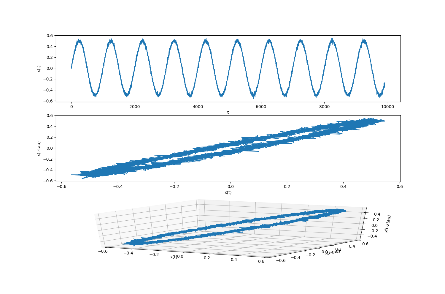
Visualize Embedding
This is how a typical sinusoidal signal looks like, when embedded in 2D and 3D respectively.
Using NeuroKit
There are different methods to guide the choice of parameters. In NeuroKit, you can use nk.complexity_optimize() to estimate the optimal parameters, including time delay, embedding dimension and tolerance threshold.
import neurokit2 as nk

signal = nk.signal_simulate(duration=10, frequency=1, noise=0.01)
parameters = nk.complexity_optimize(signal, show=True)

parameters
>>> {'delay': 13, 'dimension': 6, 'r': 0.014}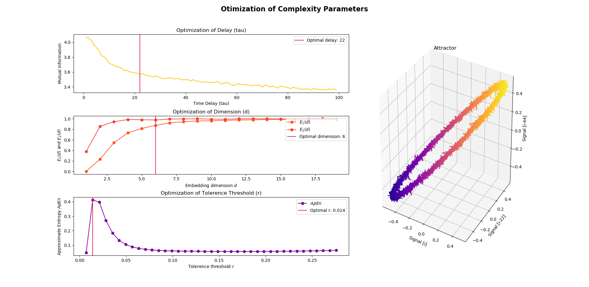
In the above example, the optimal time delay is estimated using the Mutual Information method (Fraser & Swinney, 1986), the optimal embedding dimension is estimated using the Average False Nearest Neighbour (Cao, 1997) and the optimal r is obtained using the Maximum Approximate Entropy (Lu et al., 2008). These are the default methods in nk.complexity_optimize(). Nevertheless, you can specify your preferred method via the method arguments.
More of these methods can be read about in this chapter here.
The complexity of physiological signals can be represented by the entropy of these non-linear, dynamic physiological systems.
Entropy can be defined as the measure of disorder in a signal.
- call
nk.entropy_shannon()
- Quantifies the amount of regularity and the unpredictability of fluctuations over time-series data.
- Advantages of ApEn: lower computational demand (can be designed to work for small data samples i.e. less than 50 data points and can be applied in real time) and less sensitive to noise.
- Smaller values indicate that the data is more regular and predictable, and larger values corresponding to more complexity or irregularity in the data.
- call
nk.entropy_approximate()
Examples of use
| Reference | Signal | Parameters | Findings |
|---|---|---|---|
| Caldirola et al. (2004) | 17min breath-by-breath recordings of respiration parameters | m=1, r=0.2 | Panic disorder patients showed higher ApEn indexes in baseline RSP patterns (all parameters) than healthy subjects |
| Burioka et al. (2003) | 30 mins of Respiration, 20s recordings of EEG | m=2, r=0.2, τ=1.1s for respiration, 0.09s for EEG | Lower ApEn of respiratory movement and EEG in stage IV sleep than other stages of consciousness |
| Boettger et al. (2009) | 64s recordings of QT and RR intervals | m=2, r=0.2 | Higher ratio of ApEn(QT) to ApEn(RR) for higher intensities of exercise, reflecting sympathetic activity |
| Taghavi et al. (2011) | 2mis recordings of EEG | m=2, r=0.1 | Higher ApEn of normal subjects than schizophrenic patients particularly in limbic areas of the brain |
- A modification of approximate entropy
- Advantages over ApEn: data length independence and a relatively trouble-free implementation.
- Large values indicate high complexity whereas smaller values characterize more self-similar and regular signals.
- call
nk.entropy_sample()
Examples of use
| Reference | Signal | Parameters | Findings |
|---|---|---|---|
| Lake et al. (2002) | 25min recordings of RR intervals | m=3, r=0.2 | SampEn is lower in the course of neonatal sepsis and sepsislike illness |
| Lake et al. (2011) | 24h recordings of RR intervals | m=1, r=to vary |
|
| Estrada et al. (2015) | EMG diaphragm signal | m=1, r=0.3 | fSampEn (fixed SampEn) method to extract RSP rate from respiratory EMG signal |
| Kapidzic et al. (2014) | RR intervals and its corresponding RSP signal | m=2, r=0.2 | During paced breathing, significant reduction of SampEn(Resp) and SampEn(RR) with age in male subjects, compared to smaller and nonsignificant SampEn decrease in females |
| Abásolo et al. (2006) | 5min recordings of EEG in 5 second epochs | m=1, r=0.25 | Alzheimer's Disease patients had lower SampEn than controls in parietal and occipital regions |
- Similar to ApEn and SampEn
- call
nk.entropy_fuzzy()
- Expresses different levels of either ApEn or SampEn by means of multiple factors for generating multiple time series
- Captures more useful information than using a scalar value produced by ApEn and SampEn
- call
nk.entropy_multiscale()