Niko Seino 2022-07-07
Bellabeat is a high-tech company that manufactures health-focused smart products. Collecting data on activity, sleep, stress, and reproductive health has allowed Bellabeat to empower women with knowledge about their own health and habits.
Sršen, the company’s cofounder, would like an analysis of Bellabeat’s available consumer data to identify opportunities for growth. She has asked the marketing analytics team to analyze smart device usage data in order to gain insight into how people are already using their smart devices. Then, using this information, she would like recommendations for how these trends can inform Bellabeat marketing strategy. Therefore, in this case study, I will answer the following questions:
- What are some trends in smart device usage?
- How can these trends help influence Bellabeat marketing strategy?
The data for this case study comes from Fitbit Fitness Tracker Data, a public domain dataset available on Kaggle. It contains personal fitness tracker information from 30 FitBit users. These 30 Fitbit users consented to the submission of all personal tracker data contained in this dataset.
I will import the data set from Kaggle into RStudio where I can clean, filter, and analyze the data.
- Sample size: 30 people is not a large enough sample to be representative of all FitBit users
- Outdated: The dataset contains data from a one month period in 2016 only. For a deeper and more accurate analysis of trends, we would need data from the current year, preferably collected for an entire year to look at if trends vary during different times of year.
- Limited: The dataset does not contain any demographic information about the users, including gender, age, or location, which would be beneficial for marketing purposes to target specific customers
- load packages
suppressPackageStartupMessages(library(tidyverse))
suppressPackageStartupMessages(library(ggplot2))
suppressPackageStartupMessages(library(lubridate))
suppressPackageStartupMessages(library(lm.beta))- Load CSV files containing our data
# set working directory
# setwd("~/Fitbit Case Study")
# load files
daily_activity <- read.csv("dailyActivity_merged.csv")
hourly_steps <- read.csv("hourlySteps_merged.csv")
daily_sleep <- read.csv("sleepDay_merged.csv")
weight <- read.csv("weightLogInfo_merged.csv")- Identify number of participants in each data set by counting distinct IDs
n_distinct(daily_activity$Id)## [1] 33
n_distinct(hourly_steps$Id)## [1] 33
n_distinct(daily_sleep$Id)## [1] 24
n_distinct(weight$Id)## [1] 8
Note: Because very few participants contributed weight data, we will exclude it from our analysis
- View and clean up the data sets
# First, the daily_sleep data
head(daily_sleep)
## Id SleepDay TotalSleepRecords TotalMinutesAsleep
## 1 1503960366 4/12/2016 12:00:00 AM 1 327
## 2 1503960366 4/13/2016 12:00:00 AM 2 384
## 3 1503960366 4/15/2016 12:00:00 AM 1 412
## 4 1503960366 4/16/2016 12:00:00 AM 2 340
## 5 1503960366 4/17/2016 12:00:00 AM 1 700
## 6 1503960366 4/19/2016 12:00:00 AM 1 304
## TotalTimeInBed
## 1 346
## 2 407
## 3 442
## 4 367
## 5 712
## 6 320
# The 12:00:00 AM time stamp on each observation is redundant so we should remove it to make the data easier to work with
daily_sleep$SleepDay <- (gsub('12:00:00 AM', '', daily_sleep$SleepDay))
# Renaming column
colnames(daily_sleep)[2] = "Date"
# View updated data
head(daily_sleep)
## Id Date TotalSleepRecords TotalMinutesAsleep TotalTimeInBed
## 1 1503960366 4/12/2016 1 327 346
## 2 1503960366 4/13/2016 2 384 407
## 3 1503960366 4/15/2016 1 412 442
## 4 1503960366 4/16/2016 2 340 367
## 5 1503960366 4/17/2016 1 700 712
## 6 1503960366 4/19/2016 1 304 320
# Next, the daily_activity data
head(daily_activity)
## Id ActivityDate TotalSteps TotalDistance TrackerDistance
## 1 1503960366 4/12/2016 13162 8.50 8.50
## 2 1503960366 4/13/2016 10735 6.97 6.97
## 3 1503960366 4/14/2016 10460 6.74 6.74
## 4 1503960366 4/15/2016 9762 6.28 6.28
## 5 1503960366 4/16/2016 12669 8.16 8.16
## 6 1503960366 4/17/2016 9705 6.48 6.48
## LoggedActivitiesDistance VeryActiveDistance ModeratelyActiveDistance
## 1 0 1.88 0.55
## 2 0 1.57 0.69
## 3 0 2.44 0.40
## 4 0 2.14 1.26
## 5 0 2.71 0.41
## 6 0 3.19 0.78
## LightActiveDistance SedentaryActiveDistance VeryActiveMinutes
## 1 6.06 0 25
## 2 4.71 0 21
## 3 3.91 0 30
## 4 2.83 0 29
## 5 5.04 0 36
## 6 2.51 0 38
## FairlyActiveMinutes LightlyActiveMinutes SedentaryMinutes Calories
## 1 13 328 728 1985
## 2 19 217 776 1797
## 3 11 181 1218 1776
## 4 34 209 726 1745
## 5 10 221 773 1863
## 6 20 164 539 1728
# The LoggedActivitiesDistance and SedentaryActiveDistance columns don't provide much information
#   so we will not use them in our analysis and can remove them
daily_activity <- daily_activity[c(-6, -10)]
# Renaming column
colnames(daily_activity)[2] = "Date"
# View updated Data
head(daily_activity)
## Id Date TotalSteps TotalDistance TrackerDistance
## 1 1503960366 4/12/2016 13162 8.50 8.50
## 2 1503960366 4/13/2016 10735 6.97 6.97
## 3 1503960366 4/14/2016 10460 6.74 6.74
## 4 1503960366 4/15/2016 9762 6.28 6.28
## 5 1503960366 4/16/2016 12669 8.16 8.16
## 6 1503960366 4/17/2016 9705 6.48 6.48
## VeryActiveDistance ModeratelyActiveDistance LightActiveDistance
## 1 1.88 0.55 6.06
## 2 1.57 0.69 4.71
## 3 2.44 0.40 3.91
## 4 2.14 1.26 2.83
## 5 2.71 0.41 5.04
## 6 3.19 0.78 2.51
## VeryActiveMinutes FairlyActiveMinutes LightlyActiveMinutes SedentaryMinutes
## 1 25 13 328 728
## 2 21 19 217 776
## 3 30 11 181 1218
## 4 29 34 209 726
## 5 36 10 221 773
## 6 38 20 164 539
## Calories
## 1 1985
## 2 1797
## 3 1776
## 4 1745
## 5 1863
## 6 1728
# Finally, the hourly_steps data
head(hourly_steps)
## Id ActivityHour StepTotal
## 1 1503960366 4/12/2016 12:00:00 AM 373
## 2 1503960366 4/12/2016 1:00:00 AM 160
## 3 1503960366 4/12/2016 2:00:00 AM 151
## 4 1503960366 4/12/2016 3:00:00 AM 0
## 5 1503960366 4/12/2016 4:00:00 AM 0
## 6 1503960366 4/12/2016 5:00:00 AM 0
# In this case, the time associated with the date is relevant so we don't want to remove it,
#   but the data may be easier to work with if we separate it into it's own column
hourly_steps <- hourly_steps %>% separate(ActivityHour, c("Date", "Hour"), sep = "^\\S*\\K")
# View the updated dataframe
head(hourly_steps)
## Id Date Hour StepTotal
## 1 1503960366 4/12/2016 12:00:00 AM 373
## 2 1503960366 4/12/2016 1:00:00 AM 160
## 3 1503960366 4/12/2016 2:00:00 AM 151
## 4 1503960366 4/12/2016 3:00:00 AM 0
## 5 1503960366 4/12/2016 4:00:00 AM 0
## 6 1503960366 4/12/2016 5:00:00 AM 0
Because the Id variable is currently numerical but should be treated as nominal,we need to change how it is formatted in each data set.
daily_activity$Id <- as.character(daily_activity$Id)
daily_sleep$Id <- as.character(daily_sleep$Id)
hourly_steps$Id <- as.character(hourly_steps$Id)- Graph variables of interest, check for outliers in the data
summary(daily_activity$TotalSteps)## Min. 1st Qu. Median Mean 3rd Qu. Max.
## 0 3790 7406 7638 10727 36019
ggplot(daily_activity, aes(x = TotalSteps)) +
  geom_boxplot()

# Most of the daily total steps appear to be around 4000-11000.
#   There appear to be possible outliers on the high end

steps_upper <- quantile(daily_activity$TotalSteps, .9985, na.rm = TRUE)
# This shows that 99.85% of the observations are at 28,680 or below.
# Values above this number are more than 3 standard deviations from the mean,
#   indicating they are outliers.

daily_activity <- subset(daily_activity, TotalSteps <= 28680)
# 2 outliers were removed- Extract more information by running descriptive statistics
- What is the average amount of sleep for each participant?
mean_sleep <- daily_sleep %>%
  group_by(Id) %>%
  summarize(mean_sleep = mean(TotalMinutesAsleep)) %>%
  select(Id, mean_sleep) %>%
  arrange(mean_sleep) %>%
  as.data.frame()
head(mean_sleep)
## Id mean_sleep
## 1 2320127002 61.0000
## 2 7007744171 68.5000
## 3 4558609924 127.6000
## 4 3977333714 293.6429
## 5 1644430081 294.0000
## 6 8053475328 297.0000
- What percent of the time did participants actually spend sleeping while laying in bed?
daily_sleep %>%
  group_by(Id) %>%
  mutate(percent_sleep = (TotalMinutesAsleep/TotalTimeInBed)*100) %>%
  select(Id, percent_sleep) %>%
  summarize(avg_persleep = mean(percent_sleep)) %>%
  arrange(avg_persleep) %>%
  mutate_if(is.numeric, round, 2)
## # A tibble: 24 × 2
## Id avg_persleep
## <chr> <dbl>
## 1 3977333714 63.4
## 2 1844505072 67.8
## 3 1644430081 88.2
## 4 2320127002 88.4
## 5 4558609924 90.7
## 6 2347167796 91.0
## 7 5553957443 91.5
## 8 8378563200 91.9
## 9 4445114986 92.5
## 10 4020332650 93.0
## # … with 14 more rows
# Most participants slept for at least 90% of the time they spent in bed, with
#   only 4 participants spending a smaller percent of time sleeping, the lowest
# being 63.37%- Summary stats of different activity levels:
suppressPackageStartupMessages(library(psych))

activity_level <- daily_activity[9:12]
describe(activity_level)
## vars n mean sd median trimmed mad min max
## VeryActiveMinutes 1 938 20.91 32.35 4 13.92 5.93 0 210
## FairlyActiveMinutes 2 938 13.50 19.94 6 9.32 8.90 0 143
## LightlyActiveMinutes 3 938 192.58 109.02 199 193.33 102.30 0 518
## SedentaryMinutes 4 938 991.29 301.57 1059 998.80 388.44 0 1440
## range skew kurtosis se
## VeryActiveMinutes 210 2.15 5.61 1.06
## FairlyActiveMinutes 143 2.49 8.05 0.65
## LightlyActiveMinutes 518 -0.04 -0.37 3.56
## SedentaryMinutes 1440 -0.29 -0.68 9.85
- Activity levels by participant
activity_id <- daily_activity %>%
  group_by(Id) %>%
  summarize(sum_very = sum(VeryActiveMinutes),
            sum_fairly = sum(FairlyActiveMinutes),
            sum_lightly = sum(LightlyActiveMinutes),
            sum_sed = sum(SedentaryMinutes)) %>%
  select(Id, sum_very, sum_fairly, sum_lightly, sum_sed) %>%
  as.data.frame()
head(activity_id)
## Id sum_very sum_fairly sum_lightly sum_sed
## 1 1503960366 1200 594 6818 26293
## 2 1624580081 83 117 4587 37970
## 3 1644430081 287 641 5354 34856
## 4 1844505072 4 40 3579 37405
## 5 1927972279 41 24 1196 40840
## 6 2022484408 1125 600 7981 34490
- On average, during which hour of the day were the most steps taken?
hourly_steps %>%
  group_by(Hour) %>%
  summarize(mean_steps = mean(StepTotal)) %>%
  select(Hour, mean_steps) %>%
  arrange(desc(mean_steps)) %>%
  head(1)
## # A tibble: 1 × 2
## Hour mean_steps
## <chr> <dbl>
## 1 " 6:00:00 PM" 599.
# Answer: 6:00PM with an average of about 600 steps
# Creating a dataframe with average hourly steps for later visualization
mean_steps <- hourly_steps %>%
  group_by(Hour) %>%
  summarize(mean_steps = mean(StepTotal)) %>%
  select(Hour, mean_steps) %>%
  arrange(desc(Hour)) %>%
as.data.frame()- What is the mean and standard deviation for total steps taken by participant?
steps_byId <- hourly_steps %>%
  group_by(Id) %>%
  summarize(mean_steps_id = mean(StepTotal), sd_steps_id = sd(StepTotal)) %>%
  mutate_if(is.numeric, round, 2) %>%
  as.data.frame()
head(steps_byId)
## Id mean_steps_id sd_steps_id
## 1 1503960366 522.38 836.48
## 2 1624580081 241.51 760.46
## 3 1644430081 307.81 589.61
## 4 1844505072 109.36 232.06
## 5 1927972279 38.59 164.17
## 6 2022484408 477.87 861.30
- Relationship between steps taken in a day and sedentary minutes:
ggplot(data=daily_activity, aes(x=TotalSteps, y=SedentaryMinutes)) +
  geom_point() +
  geom_smooth() +
  labs(title="Total Steps vs. Sedentary Minutes",
       x = "Steps", y = "Minutes")

There appears to be no correlation between total daily steps taken and sedentary minutes. We can confirm with a simple linear regression:
sed_steps_lr <-lm(SedentaryMinutes ~ TotalSteps, daily_activity)
summary(sed_steps_lr)
##
## Call:
## lm(formula = SedentaryMinutes ~ TotalSteps, data = daily_activity)
##
## Residuals:
## Min 1Q Median 3Q Max
## -1145.7 -234.3 103.0 240.8 539.1
##
## Coefficients:
## Estimate Std. Error t value Pr(>|t|)
## (Intercept) 1.146e+03 1.697e+01 67.53 <2e-16 ***
## TotalSteps -2.041e-02 1.873e-03 -10.89 <2e-16 ***
## ---
## Signif. codes: 0 '***' 0.001 '**' 0.01 '*' 0.05 '.' 0.1 ' ' 1
##
## Residual standard error: 284.2 on 936 degrees of freedom
## Multiple R-squared: 0.1125, Adjusted R-squared: 0.1116
## F-statistic: 118.7 on 1 and 936 DF, p-value: < 2.2e-16
Results confirm little correlation, with an r^2 value of .11
- Average amount of time participants slept each night during the course of the study:
# Graph the results
options(scipen = 999)
ggplot(mean_sleep, aes(x = Id, y = mean_sleep)) +
  geom_col(aes(reorder(Id, +mean_sleep), y = mean_sleep)) +
  labs(title = "Average Minutes of Sleep", x = "Participant Id", y = "Minutes") +
  theme(axis.text.x = element_text(angle = 90)) +
  geom_hline(yintercept = mean(mean_sleep$mean_sleep), color = "red")

The graph shows the average sleep of each participant individually, as well as how their sleep compares to the overall average across all participants.
- Average steps per hour:
ggplot(mean_steps, aes(x = Hour, y = mean_steps)) +
  geom_col(aes(reorder(Hour, +mean_steps), mean_steps)) +
  theme(axis.text.x = element_text(angle = 90)) +
  labs(title = "Average Steps Taken per Hour of Day",
       x = "Hour", y = "Average Steps")

We can see that the most steps were taken in the evening, from 5-7pm, and the least steps in the middle of the night, between 12-4am.
- I’m going to combine two datasets I created previously, activity_id and steps_byId, in order to find new relationships between variables.
combined_data <- merge(activity_id, steps_byId, by = "Id")

# Putting just the numerical variables into a separate dataframe, then running a correlation matrix
num_data <- combined_data[-1]
cor(num_data)
## sum_very sum_fairly sum_lightly sum_sed mean_steps_id
## sum_very 1.00000000 0.3310092 0.08229265 -0.01609547 0.6978256
## sum_fairly 0.33100923 1.0000000 0.12218239 -0.14896700 0.4695951
## sum_lightly 0.08229265 0.1221824 1.00000000 -0.02534821 0.5080046
## sum_sed -0.01609547 -0.1489670 -0.02534821 1.00000000 -0.1968506
## mean_steps_id 0.69782565 0.4695951 0.50800458 -0.19685056 1.0000000
## sd_steps_id 0.71214478 0.4478268 0.25023909 -0.04474601 0.9126453
## sd_steps_id
## sum_very 0.71214478
## sum_fairly 0.44782678
## sum_lightly 0.25023909
## sum_sed -0.04474601
## mean_steps_id 0.91264532
## sd_steps_id 1.00000000
# Based on the correlation matrix, there is little correlation between the different activity levels, but there is a moderate (.7) correlation between mean steps taken and very active minutes.

ggplot(combined_data, aes(x = mean_steps_id, y = sum_very)) +
  geom_point() +
  labs(title = "Average Steps Taken in a Day Compared to Very Active Minutes",
       x = "Average Steps", y = "Very Active Minutes")

We can see a moderate upwards trend of “very active minutes” increasing as average steps in a day increases.
- I completed additional visualizations in Tableau, which can be viewed here: Bellabeat Dashboard - Tableau
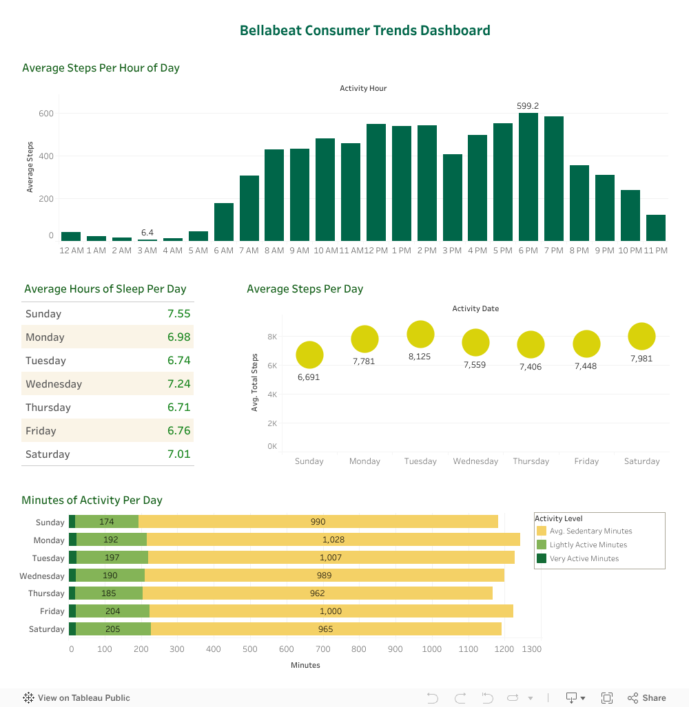
The descriptive statistical analyses and visualizations completed show the following smart device usage trends:
- Sedentary minutes took up the majority of participants’ days and were fairly consistent throughout the week.
- Average “very active minutes” were also consistent throughout the week at around 20 minutes each day.
- On average, participants slept the most on Sundays, which was also the day they took the least amount of steps
- Participants took the most steps on Tuesdays and Saturdays.
- On average, the fewest steps were taken at 3:00 and the most steps taken at 18:00
- On average, participants slept about 390 minues, or 6.5 hours per night
- Users who take more steps per day are more likely to engage in “very active minutes”
How can these trends help influence Bellabeat marketing strategy?
We can make marketing recommendations based on what we have learned about how customers are currently using smart fitness devices:
-
Very few customers utilized the weight log feature, so this does not appear to be a selling point. Focus on marketing other features such as activity, sleep, and steps tracking, and consider further research into how to make the weight log feature more marketable
-
Our data shows that when active, participants engaged the most in “light” activity and did not have many “very active” minutes each day. The company could add a “level up” feature in which participants can earn points based on time spent being active, with higher levels of activity earning more points. This could motivate users to engage in active minutes more often.
-
There’s about a 1000 step decrease on Sundays compared to the other days of the week. A notification on Sunday mornings with a goal to hit a certain number of steps, along with a reward for hitting a 7-day streak could help close this gap and encourage customers to use the device all days of the week.
-
Based on data showing the most usage around 6pm, it seems likely most users have typical work hours during the day and get most of their steps in after work. An ad targeted towards working adults focused on easily tracking steps throughout their busy days could be effective. A reminder notification around 12pm and 8pm can encourage users to increase their activity levels during other break times such as lunch and after dinner as well.
-
On average, participants got less than the CDC recommended 7 hours of sleep per night. Continue marketing the device’s sleep tracking feature as participants who are not getting enough sleep may want a way to track their sleep patterns. Consider marketing along with a meditation app or habit tracker.