
Write a software pipeline to detect vehicles in a video.
Steps of this project are the following:
- Perform a Histogram of Oriented Gradients (HOG) feature extraction on a labeled training set of images
- Apply a color transform and append binned color features, as well as histograms of color, to HOG feature vector.
- Normalize features
- Split training and testing data
- Train a classifier using Linear SVC classifier
- Implement a sliding-window technique and use trained classifier to search for vehicles in images.
- Create heatmap of recurring detections frame by frame and remove false positives by thresholding number of windows found
- Combine multiple boxes into a single one detected for a single car
- Verify pipeline on test images
- Run pipeline on a video stream
Here are links to the labeled data for vehicle and non-vehicle examples to train our classifier. These example images come from a combination of the GTI vehicle image database, the KITTI vision benchmark suite, and examples extracted from the project video itself.
Let's start!
First step is to read and store car and non-car images for training
cars = glob.glob('vehicles/*/*.png')
notcars = glob.glob('non-vehicles/*/*.png')

[Code for this section is in color_hist() method]
Template matching are not robust to changes in appearance, hence we use a better transformation method which is to compute histogram of color values, this gives locations of similar distribution a close match therefore removing sensitiviting to perfect arrangement of pixels.
We can construct histograms of the R, G, and B channels like this:
  rhist = np.histogram(image[:,:,0], bins=32, range=(0, 256))
  ghist = np.histogram(image[:,:,1], bins=32, range=(0, 256))
  bhist = np.histogram(image[:,:,2], bins=32, range=(0, 256))
Results of plotting for car image:

Results of plotting for non-car image:

Disadvantage of histogram of color transformation is we are purely relying on color.
[Code for this section is in plot3d() method]
Cars are more saturated than background like sky, road, etc., hence we will explore different color spaces (RGB, HSV, YCrRB) and also we will check the difference between choosen color space for car image and non car image.
From results of various color spaces we can observe that it is easy to differentiate different colors using YCrRB:


[Code for this section is in bin_spatial() method]
Raw pixel values are still quite useful to include in our feature vector in searching for cars. As it will be cumbersome to include three color channels of a full resolution image we can perform spatial binning on an image and still retain enough information to help in finding vehicles.
Even going all the way down to 32 x 32 pixel resolution, the car itself will still be clearly identifiable by eye, and this means that the relevant features are still preserved at this resolution.
small_img = cv2.resize(image, (32, 32))

[Code for this section is in get_hog_features() method]
Gradients and edges gives more robust representation and captures notion of shape.
There is an excellent tutorial here: http://www.learnopencv.com/histogram-of-oriented-gradients/ but we will list few important terms here:
In the HOG feature descriptor, the distribution (histograms) of directions of gradients (oriented gradients) are used as features. Gradients (x and y derivatives) of an image are useful because the magnitude of gradients is large around edges and corners (regions of abrupt intensity changes) and we know that edges and corners pack in a lot more information about object shape than flat regions.
At every pixel, the gradient has a magnitude and a direction. We will group these pixels into small cells (say 8 x8 pixels). Inside these cell will compute HOG. The x-gradient fires on vertical lines and the y-gradient fires on horizontal lines. The magnitude of gradient fires where ever there is a sharp change in intensity. None of them fire when the region is smooth.
For color images, the gradients of the three channels are evaluated. The magnitude of gradient at a pixel is the maximum of the magnitude of gradients of the three channels, and the angle is the angle corresponding to the maximum gradient.
The histogram is essentially a vector (or an array ) of 9 bins (numbers) corresponding to angles 0, 20, 40, 60 … 160. Gradient samples are distributed into these bins and summed up.
Each pixel in the image gets a vote on which histogram bin it belongs based on the gradient direction at that position, but the weight of that vote depends on the gradient magnitude at that pixel. When we do this for all the cells we see a representation of the original strucutre image, this can be used as a signature for a given shape; like these for car:


HOG for non-car:

The scikit-image package has a built in function to extract Histogram of Oriented Gradient features:
The scikit-image hog() function takes in a single color channel or grayscaled image as input, as well as parameters like orientations, pixels_per_cell and cells_per_block.
Orientations:
- The number of orientations is specified as an integer, and represents the number of orientation bins that the gradient information will be split up into in the histogram.
- Typical values are between 6 and 12 bins. To encode finer orientation details, increase the number of bins. Increasing this value increases the size of the feature vector, which requires more time to process.
Pixels-per-cell:
- The pixels_per_cell parameter specifies the cell size over which each gradient histogram is computed. This paramater is passed as a 2-tuple so we could have different cell sizes in x and y, but cells are commonly chosen to be square.
- To capture large-scale spatial information, increase the cell size. When we increase the cell size, we may lose small-scale detail.
Cells-per-block:
-
The cells_per_block parameter is also passed as a 2-tuple, and specifies the local area over which the histogram counts in a given cell will be normalized.
-
Reducing the block size helps to capture the significance of local pixels. Smaller block size can help suppress illumination changes of HOG features.
from skimage.feature import hog
def get_hog_features(img, orient, pix_per_cell, cell_per_block, vis=False, feature_vec=True):
    if vis == True:
        features, hog_image = hog(img, orientations=orient, pixels_per_cell=(pix_per_cell, pix_per_cell),
                                  cells_per_block=(cell_per_block, cell_per_block), transform_sqrt=False,
                                  visualise=True, feature_vector=False)
        return features, hog_image
    else:
        features = hog(img, orientations=orient, pixels_per_cell=(pix_per_cell, pix_per_cell),
                       cells_per_block=(cell_per_block, cell_per_block), transform_sqrt=False,
                       visualise=False, feature_vector=feature_vec)
        return features
Let's say we are computing HOG features for an image that is 64×64 pixels. If we set pixels_per_cell=(8, 8) and cells_per_block=(2, 2) and orientations=9. The HOG features for all cells in each block are computed at each block position and the block steps across and down through the image cell by cell. So, the actual number of features in our final feature vector will be the total number of block positions multiplied by the number of cells per block, times the number of orientations, or in the case shown above: 7×7×2×2×9=1764.
[Code for normalization is shown below and code for extracting features section is in extract_features() method]
Variety of features helps us in roboust detection system hence we first normalize all these features and then combine them.
# Create an array stack of feature vectors
X = np.vstack((car_features, notcar_features)).astype(np.float64)
# Fit a per-column scaler
X_scaler = StandardScaler().fit(X)
# Apply the scaler to X
scaled_X = X_scaler.transform(X)
Code for combining spatial, histogram of colors and hog features:
def extract_features(imgs, cspace='RGB', spatial_size=(32, 32), hist_bins=32, hist_range=(0, 256),
  orient=9, pix_per_cell=8, cell_per_block=2, hog_channel=0,
   spatial_feat=True, hist_feat=True, hog_feat=True):

      # Create a list to append feature vectors to
      features = []
      # Iterate through the list of images
      for file in imgs:
         combined_features = []
          # Read in each one by one
          image = mpimg.imread(file, format='PNG')
          # apply color conversion if other than 'RGB'
          feature_image = convert_color(image, conv='RGB2YCrCb')

          if spatial_feat:
             # Apply bin_spatial() to get spatial color features
              spatial_features = bin_spatial(feature_image, size=spatial_size)
              combined_features.append(spatial_features)
          if hist_feat:
             # Apply color_hist() also with a color space option now
              rhist, ghist, bhist, bin_centers, hist_features = color_hist(feature_image, nbins=hist_bins, bins_range=hist_range)
              combined_features.append(hist_features)
          if hog_feat:
             # Call get_hog_features() with vis=False, feature_vec=True
              if hog_channel == 'ALL':
                 hog_features = []
                  for channel in range(feature_image.shape[2]):
                     hog_features.append(get_hog_features(feature_image[:,:,channel], orient, pix_per_cell, cell_per_block, vis=False, feature_vec=True))
                  hog_features = np.ravel(hog_features)
              else:
                 hog_features = get_hog_features(feature_image[:,:,hog_channel], orient, pix_per_cell, cell_per_block, vis=False, feature_vec=True)
              combined_features.append(hog_features)

          # Append the new feature vector to the features list
          features.append(np.concatenate(combined_features))
      # Return list of feature vectors
      return features
[Code for this part is in 'Classifier' section of notebook]
-
Extract features (color and hog features) from list of images
-
Combine features
-
Shuffle the input data (provided) - to avoid problems due to overfitting
-
Split the data into training and testing set - to avoid overfitting and improve generalization:
from sklearn.cross_validation import train_test_split rand_state = np.random.randint(0, 100) X_train, X_test, y_train, y_test = train_test_split( scaled_X, y, test_size=0.2, random_state=rand_state) -
Define output lables:
y = np.hstack((np.ones(len(car_features)), np.zeros(len(notcar_features)))) -
Train a classifier to detect car images from other images using LinearSVC() (I experimented other classifiers but finally considered this LinearSVC() was simple, fast and gave accuracy of more than 98%)
` from sklearn.svm import LinearSVC svc = LinearSVC() svc.fit(X_train, y_train) -
Check accuracy
print('Test Accuracy of SVC = ', svc.score(X_test, y_test)) -
Predict output: We can test predicted output using below code:
print('My SVC predicts: ', svc.predict(X_test[0:10].reshape(1, -1))) print('For labels: ', y_test[0:10]) -
Final step is to experiment with different parameters (Tweaked different parameters and finally settled with below parameters as with these accuracy was high and false postivies were minimum)
 color_space = 'YCrCb' # Can be RGB, HSV, LUV, HLS, YUV, YCrCb
 orient = 9  # HOG orientations
 pix_per_cell = 8 # HOG pixels per cell
 cell_per_block = 2 # HOG cells per block
 hog_channel = "ALL" # Can be 0, 1, 2, or "ALL"
 spatial_size = (32, 32) # Spatial binning dimensions
 hist_bins = 32    # Number of histogram bins
 spatial_feat = True # Spatial features on or off
 hist_feat = True # Histogram features on or off
| Color channel | HOG channel | Feature vectors | Orientations | Extraction time | Training time | Prediction time | Accuracy |
|---|---|---|---|---|---|---|---|
| HSV | All | 8460 | 9 | 66.22 | 4.11 | 0.00163 | 99.04% |
| YCrCb | 0 | 8460 | 9 | 29.6 | 13.42 | 0.00162 | 98.73% |
| YCrCb | All | 8460 | 9 | 65.83 | 3.07 | 0.00201 | 99.27% |
| YCrCb | All | 10224 | 12 | 63.47 | 3.26 | 0.00221 | 99.41% |
| RGB | All | 8460 | 9 | 60.24 | 16.8 | 0.00201 | 99.16% |
*Time in seconds
-
Save the model in a pickle file
import pickle
hist_range = (0, 256)
dist_pickle = {}
dist_pickle["svc"] = svc
dist_pickle["scaler"] = X_scaler
dist_pickle["color_space"] = color_space
dist_pickle["orient"] = orient
dist_pickle["pix_per_cell"] = pix_per_cell
dist_pickle["cell_per_block"] = cell_per_block
dist_pickle["hog_channel"] = hog_channel
dist_pickle["spatial_size"] = spatial_size
dist_pickle["hist_bins"] = hist_bins
dist_pickle["hist_range"] = hist_range

with open('svc_pickle.p', 'wb') as f:
   pickle.dump(dist_pickle, f)
Saved model can retrived using:
  dist_pickle = pickle.load(open("svc_pickle.p", "rb"))
  svc = dist_pickle["svc"]
  # and so on ....
[Code for this part is in find_cars () method of notebook]
- If accuracy is good then we will run this classifier across entire frame sampling small patches to detect presence of car in a grid pattern.
- From our successful prediction we can get start and stop positions in both x and y to get co-ordinates of bounding boxes.
- From this list of bounding boxes for the search windows we can draw rectangles using draw draw_boxes() function.
Instead of extracting hog features for every small patch, we will extract hog features once and sub small to get all windows/boxes.
Car predicted using a classifier and drawn rectangle over predicted cars:

[Code for this part is in pipleline () method of notebook]
The multi-scale window approach prevents calculation of feature vectors for the complete image and thus helps in speeding up the process.
We are not sure what's the scale of the image we are searching (for example: cars far away appear smaller and closes ones appear large) hence we will set few minimum, maximum and intermediate scales to search.
for scale in scales:
   box_list += find_cars(img, ystart, ystop, scale, svc, X_scaler, color_space, orient, pix_per_cell, cell_per_block, hog_channel, spatial_size, hist_bins, hist_range)
See what happens when scale is 1.25:

See what happens when scale is 1.5:

We will also choose different ystop/ystart along scales in our pipeline (see below) to effecitively search our cars.
[Code for this part is in 'multiple detections and false postives' section of notebook]
As seen below we will get multiple detections for the same car and also a false positives (i.e., classifier predicted a car where was no car), we should filter these out:

For this, we will build a heat map to combine overlapping detections and remove false positives:
Step 1: To make a heat-map, we're simply going to add "heat" (+=1) for all pixels within windows where a positive detection is reported by our classifier.
Heat map with both multiple detections False postive:

Step 2: Due to above, areas of multiple detections get "hot", while transient false positives stay "cool". We can then simply threshold our heatmap to remove false positives. Ex: heatmap = threshold(heatmap, 4) # if number of detected windows are less than 4 than those will be considered as false positive.
Thresholded heatmap:

Step 3: To figure out how many cars we have in each frame and which pixels belong to which cars, we use the label() function from scipy.ndimage.measurements.
Step 4: We can take our thresholded and labeled images and put bounding boxes around the labeled regions, so that we get single box instead of multiple detections for the same car - this we will our output image.

Code:
from scipy.ndimage.measurements import label

def add_heat(img, bbox_list):
    heatmap = np.zeros_like(img[:,:,0]).astype(np.float)
    # Iterate through list of bboxes
    for box in bbox_list:
        # Add += 1 for all pixels inside each bbox
        heatmap[box[0][1]:box[1][1], box[0][0]:box[1][0]] += 1
    # Return updated heatmap
    return np.clip(heatmap, 0, 255)

def apply_threshold(heatmap, threshold):
    heat = np.copy(heatmap)
    # Zero out pixels below the threshold
    heat[heat <= threshold] = 0
    # Return thresholded map
    return heat

def draw_labeled_bboxes(img, labels):
    # Make a copy of the image
    imcopy = np.copy(img)
    # Iterate through all detected cars
    for car_number in range(1, labels[1]+1):
        # Find pixels with each car_number label value
        nonzero = (labels[0] == car_number).nonzero()
        # Identify x and y values of those pixels
        nonzeroy = np.array(nonzero[0])
        nonzerox = np.array(nonzero[1])
        # Define a bounding box based on min/max x and y
        bbox = ((np.min(nonzerox), np.min(nonzeroy)), (np.max(nonzerox), np.max(nonzeroy)))
        # Draw the box on the image
        cv2.rectangle(imcopy, bbox[0], bbox[1], (0,0,255), 6)
    # Return the image
    return imcopy
Once we are comfortable with our output on a single image we can test on series of images:
def pipeline(img):
scales = [1.0, 1.25, 1.5, 1.75, 2.]
box_list = []
# Experiment with ystart, ystop and scale values
for (ystart, ystop, scale) in [(380, 580, 1), (400, 500, 1.3) , (420, 600, 1.5), (400, 650, 1.7), (450, 680, 2)]:
    box_list += find_cars(img, ystart, ystop, scale, svc, X_scaler, color_space, orient, pix_per_cell, cell_per_block, hog_channel, spatial_size, hist_bins, hist_range)
    heatmap = add_heat(img, box_list)
    updated_heatmap = apply_threshold(heatmap, 5)
    labels = label(updated_heatmap)
    result = draw_labeled_bboxes(img, labels)
return result


Final step will be to run on project video:
from moviepy.editor import VideoFileClip
from IPython.display import HTML

video_output = 'project_video_output.mp4'
clip1 = VideoFileClip("project_video.mp4")
video_clip = clip1.fl_image(pipeline)
%time video_clip.write_videofile(video_output, audio=False)
Here we will combine the lane detection (project #4) and vehicle detection pipeline test on our project_video.
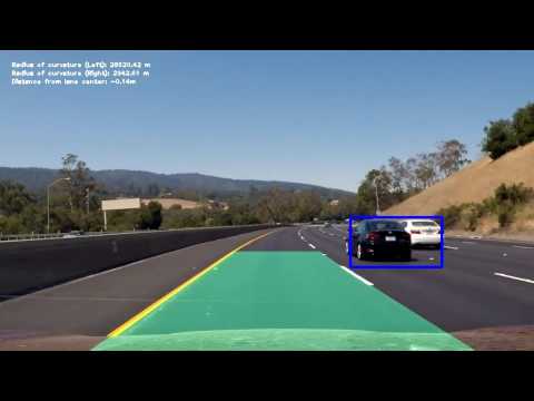
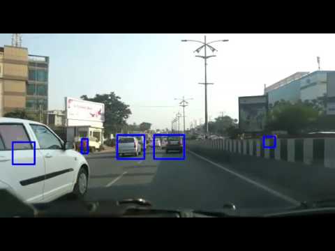
Below is video of vehicle detection pipeline running on video which I recorded for this project; results are not accurate but still does a decent job that too without changing any part of the code; we can see that it has detected cars most of the times (and as expected not detected other vehicles).
Future work:
-
Optimize search by limiting number of frames to search, instead of processing for every frame.
-
Remove false postivies.
-
Make car detection smooth - in the above pipeline bounding boxes keeps jumping around.
-
Try similar pipepline but using Deep learning with VGG-16 pre-trained model for Keras.
References: