DPFEHM is a Julia module that includes differentiable numerical models with a focus on the Earth's subsurface, especially fluid flow. Currently it supports the groundwater flow equations (single phase flow), Richards equation (air/water), the advection-dispersion equation, and the 2d wave equation. Since it is differentiable, it can easily be combined with machine learning models in a workflow such as this:

This workflow shows how to train a machine learning model to mitigate problems with injecting fluid into the earth's subsurface (such as induced seismicity or leakage of carbon dioxide). More details on this workflow are available here.
Within Julia, you can install DPFEHM and test that it works by running
import Pkg
Pkg.add("DPFEHM")
Pkg.test("DPFEHM")The examples are a good place to get started to see how to use DPFEHM. Two examples will be described in detail here that illustrate the basic usage patterns via an examples of steady-state single-phase flow and transient Richards equation.
Here, we solve a steady-state single phase flow problem . Let's start by importing several libraries that we will use.
import DPFEHM
import GaussianRandomFields
import Optim
import PyPlot
import Random
import Zygote
Random.seed!(0)#set the seed so we can reproduce the same results with each run
Next, we'll set up the grid. Here, we use a regular grid with 100,000 nodes that covers a domain that is 50 meters by 50 meters by 5 meters.
mins = [0, 0, 0]; maxs = [50, 50, 5]#size of the domain, in meters
ns = [100, 100, 10]#number of nodes on the grid
coords, neighbors, areasoverlengths, _ = DPFEHM.regulargrid3d(mins, maxs, ns)#build the grid
The result of this grid-building is three variables that we will use. The, coords is a matrix describing the coordinates of the cell centers on the grid. The second, neighbors, is an array describing which cells neighbor other cells. The third, areasoverlengths, is another array whose length is equal to the length of neighbors and describes the area of the interface between two neighboring cells dividing by the length between the cell centers. The last variable is dumped to _ and gives the volumes of the cells. The volumes of the cells are not needed for steady state problems, so they are not used in this example.
Now we set up the boundary conditions.
Qs = zeros(size(coords, 2))
injectionnode = 1#inject in the lower left corner
Qs[injectionnode] = 1e-4#m^3/s
dirichletnodes = Int[size(coords, 2)]#fix the pressure in the upper right corner
dirichleths = zeros(size(coords, 2))
dirichleths[size(coords, 2)] = 0.0
The variable Qs describes fluid sources/sinks -- the amount of fluid injected at cell i on the grid is given by Qs[i]. In this example, the only place were we inject fluid is at node 1. Another variable, dirichletnodes is a list of cells at which the pressure will be fixed. In this example, the pressure is fixed at the last cell, which is cell number size(coords, 2). The variable dirichleths describes the pressures (or heads in hydrology jargon) that the cells are fixed at. Note that the length of dirichleths is size(coords, 2), but these values are ignored except at the indices that appear in dirichletnodes.
The final set-up step before moving on to solving the equations is to construct a heterogeneous conductivity field.
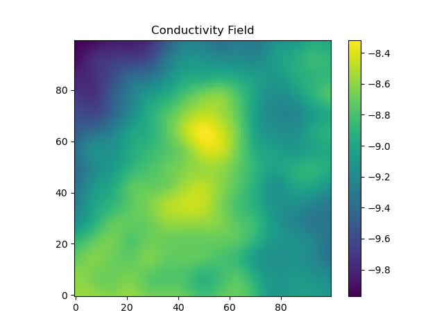
Here, we use the package GaussianRandomFields to construct a conductivity field with a correlation length of 50 meters. The mean of the log-conductivity is 1e-4meters/second (note that we use a natural logarithm when defining this), and the standard deviation of the log-conductivity is 1. GaussianRandomFields is used to construct a field in 2 dimensions and then it is copied through each of the layers, so that the heterogeneity only exists in the x and y coordinate directions, but not in the z direction.
lambda = 50.0#meters -- correlation length of log-conductivity
sigma = 1.0#standard deviation of log-conductivity
mu = -9.0#mean of log conductivity -- ~1e-4 m/s, like clean sand here https://en.wikipedia.org/wiki/Hydraulic_conductivity#/media/File:Groundwater_Freeze_and_Cherry_1979_Table_2-2.png
cov = GaussianRandomFields.CovarianceFunction(2, GaussianRandomFields.Matern(lambda, 1; σ=sigma))
x_pts = range(mins[1], maxs[1]; length=ns[1])
y_pts = range(mins[2], maxs[2]; length=ns[2])
num_eigenvectors = 200
grf = GaussianRandomFields.GaussianRandomField(cov, GaussianRandomFields.KarhunenLoeve(num_eigenvectors), x_pts, y_pts)
logKs = zeros(reverse(ns)...)
logKs2d = mu .+ GaussianRandomFields.sample(grf)'#generate a random realization of the log-conductivity field
for i = 1:ns[3]#copy the 2d field to each of the 3d layers
	v = view(logKs, i, :, :)
	v .= logKs2d
end
The conductivity field is shown:
Now, we look to solve the flow problem. First, we define a helper function, logKs2Ks_neighbors. This function is needed because the flow solver wants to know the conductivity on the interface between two cells, but our previous construction defined the conductivities at the cells themselves. It also converts from log-conductivity to conductivity and uses the geometric mean to move from the cells to the interfaces. The heart of this code is the call to DPFEHM.groundwater_steadystate, which solves the single phase steady-state flow problem that we pose. The solveforh function calls this function and returns the result after reshaping.
logKs2Ks_neighbors(Ks) = exp.(0.5 * (Ks[map(p->p[1], neighbors)] .+ Ks[map(p->p[2], neighbors)]))#convert from permeabilities at the nodes to permeabilities connecting the nodes
function solveforh(logKs, dirichleths)
	@assert length(logKs) == length(Qs)
	Ks_neighbors = logKs2Ks_neighbors(logKs)
	return reshape(DPFEHM.groundwater_steadystate(Ks_neighbors, neighbors, areasoverlengths, dirichletnodes, dirichleths, Qs), reverse(ns)...)
	end
end
With this function in hand, we can solve the problem using the solveforh wrapper function we previously defined. This function requires us to explicitly pass in logKs (the hydraulic conductivity) and dirichleths (the fixed-head boundary condition), but the other inputs to DPFEHM.groundwater_steadystate are fixed to global values.
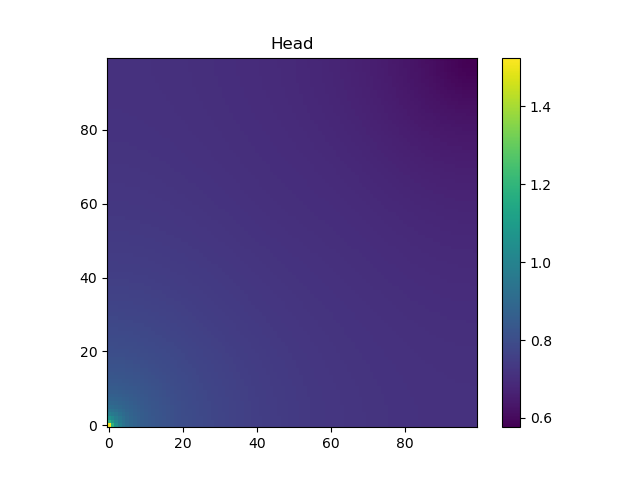
h = solveforh(logKs, dirichleths)#solve for the headThe head at the bottom layer of the domain is shown (note the pressure is higher in the lower corner, where there is fluid injection, than in the rest of the domain):
DPFEHM also allows us to compute the gradient of functions involving DPFEHM.groundwater_steadystate using Zygote.gradient or Zygote.pullback.
isfreenode, nodei2freenodei, freenodei2nodei = DPFEHM.getfreenodes(length(dirichleths), dirichletnodes)
gradient_node = nodei2freenodei[div(size(coords, 2), 2) + 500]
gradient_node_x = coords[1, gradient_node]
gradient_node_y = coords[2, gradient_node]
grad = Zygote.gradient((x, y)->solveforh(x, y)[gradient_node], logKs, dirichleths)#calculate the gradient (which involves a redundant calculation of the forward pass)
function_evaluation, back = Zygote.pullback((x, y)->solveforh(x, y)[gradient_node], logKs, dirichleths)#this pullback thing lets us not redo the forward pass
print("gradient time")
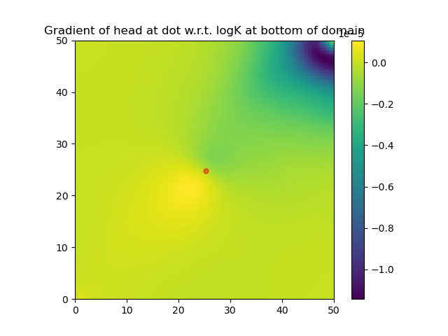
grad2 = back(1.0)#compute the gradient of a function involving solveforh using Zygote.pullbackNote that the function DPFEHM.getfreenodes allows one to map indices between the free nodes (i.e., the ones that do not have fixed-pressure boundary conditions) and all nodes. The gradient of logK at the bottom layer of the domain is shown:
Now, we consider an example using DPFEHM's solver for Richards equation, which can be used to model flow in a porous medium where both air and water fill the pores (i.e., unsaturated flow). This example is similar to the previous example and we again start by importing several libraries, setting up the grid (lower resolution this time), the boundary conditions, and the conductivity.
import DifferentiableBackwardEuler
import DPFEHM
import GaussianRandomFields
import PyPlot
import Random
import Zygote
Random.seed!(0)#set the seed so we get the same permeability over and over

#set up the grid
mins = [0, 0, 0]; maxs = [50, 50, 5]#size of the domain, in meters
ns = [30, 30, 3]#number of nodes on the grid
coords, neighbors, areasoverlengths, volumes = DPFEHM.regulargrid3d(mins, maxs, ns)#build the grid

#set up the boundary conditions
Qs = zeros(size(coords, 2))
injectionnode = 1#inject in the lower left corner
Qs[injectionnode] = 1e-4#m^3/s
dirichletnodes = Int[size(coords, 2)]#fix the pressure in the upper right corner
dirichleths = zeros(size(coords, 2))
dirichleths[size(coords, 2)] = 0.0

#set up the conductivity field
lambda = 50.0#meters -- correlation length of log-conductivity
sigma = 1.0#standard deviation of log-conductivity
mu = -9.0#mean of log conductivity -- ~1e-4 m/s, like clean sand here https://en.wikipedia.org/wiki/Hydraulic_conductivity#/media/File:Groundwater_Freeze_and_Cherry_1979_Table_2-2.png
cov = GaussianRandomFields.CovarianceFunction(2, GaussianRandomFields.Matern(lambda, 1; σ=sigma))
x_pts = range(mins[1], maxs[1]; length=ns[1])
y_pts = range(mins[2], maxs[2]; length=ns[2])
num_eigenvectors = 200
grf = GaussianRandomFields.GaussianRandomField(cov, GaussianRandomFields.KarhunenLoeve(num_eigenvectors), x_pts, y_pts)
logKs = zeros(reverse(ns)...)
logKs2d = mu .+ GaussianRandomFields.sample(grf)'#generate a random realization of the log-conductivity field
for i = 1:ns[3]#copy the 2d field to each of the 3d layers
	v = view(logKs, i, :, :)
	v .= logKs2d
end
Since we'll be solving a time-dependent problem this time, we must set the initial condition and define a storage parameter. Note that in unsaturated flows the storage parameter is often neglected (and this can be achieved by setting specificstorage to an array of ones), but this problem involves a saturated flow so we include it here. Since this is a multi-phase flow problem, we also need to define a couple parameters that control the hydraulic conductivity's dependence on the saturation. The conductivity is given by the conductivity when saturated multiplied by a relative permeability (which depends on the saturation and varies between 0 and 1).
#set up the initial condition, the storage, and the van genuchten parameters for relative permeability
h0 = zeros(size(coords, 2))#initial condition
specificstorage = fill(0.1, size(coords, 2))#storage
alphas = fill(0.5, length(neighbors))#van genuchten relative permeability parameters
Ns = fill(1.25, length(neighbors))
With the basic description of the problem complete, now we can start to write the code for solving the equations. Note that the solveforh function does not call DPFEHM.richards_steadystate to solve the equations, and instead calls DifferentiableBackwardEuler.steps. The first argument to DifferentiableBackwardEuler.steps is the initial condition, but only at the nodes that are not controlled by the Dirichlet boundary conditions. The most important parts of this call are f_richards, f_richards_u, and f_richards_p, which we will describe in the next paragraph. The argument 0.0 is the initial time, and 60 * 60 * 24 * 365 * 1 gives the simulation time (in seconds, so 1 year). The keyword arguments will eventually be passed to DifferentialEquations.solve. The last step adds the boundary conditions back into the solution, which is needed since DifferentiableBackwardEuler.steps only solves the equations on the free nodes (i.e, the nodes where the pressure is not fixed by the boundary conditions).
logKs2Ks_neighbors(Ks) = exp.(0.5 * (Ks[map(p->p[1], neighbors)] .+ Ks[map(p->p[2], neighbors)]))#convert from permeabilities at the nodes to permeabilities at the interface between nodes using the geometric mean
isfreenode, nodei2freenodei, freenodei2nodei = DPFEHM.getfreenodes(length(Qs), dirichletnodes)
function solveforh(logKs, dirichleths)
	@assert length(logKs) == length(Qs)
	Ks_neighbors = logKs2Ks_neighbors(logKs)
	p = [Ks_neighbors; dirichleths]
	h_richards = DifferentiableBackwardEuler.steps(h0[isfreenode], f_richards, f_richards_u, f_richards_p, f_richards_t, p, 0.0, 60 * 60 * 24 * 365 * 1; abstol=1e-1, reltol=1e-1)
	h_with_bcs = hcat(map(i->DPFEHM.addboundaryconditions(h_richards[:, i], dirichletnodes, dirichleths, isfreenode, nodei2freenodei), 1:size(h_richards, 2))...)#add the dirichlet boundary conditions back
	return h_with_bcs
end
Now, we define the key functions f_richards, f_richards_u, and f_richards_p from the previous paragraph. The function f_richards basically tells DifferentiableBackwardEuler to solve du/dt=f_richards and this is the function richards_residuals. The function f_richards_u is the Jacobian of f_richards with respect to the variable that is being integrated by DifferentiableBackwardEuler. We can compute the Jacobian of richards_residuals with respect to any of its inputs using the function DPFEHM.richards_XYZ where XZY is the name of the argument (as defined within DPFEHM). In the jargon of DPFEHM's Richards equation solve, the variable we are solving for is named psi, so f_richards_u just unpacks the parameters and calls DPFEHM.richards_psi. The function f_richards_p is the Jacobian of f_richards with respect to the parameter p. Since p consists of Ks and dirichleths (or dirichletpsis in the jargon of DPFEHM's Richards solver), we concatenate the two Jacobians DPFEHM.richards_Ks and DPFEHM.richards_dirichletpsis. The last function f_richards_t is currently unused, but in principle should give the Jacobian of f_richards with respect to t.
#set up some functions needed by DifferentiableBackwardEuler
function f_richards(u, p, t)#tells DifferentiableBackwardEuler to solve du/dt=f_richards
	Ks, dirichleths = unpack(p)
	return DPFEHM.richards_residuals(u, Ks, neighbors, areasoverlengths, dirichletnodes, dirichleths, coords, alphas, Ns, Qs, specificstorage, volumes)
end
function f_richards_u(u, p, t)#give DifferentiableBackwardEuler the derivative of f_richards with respect to u -- needed for the backward euler method that we use
	Ks, dirichleths = unpack(p)
	return DPFEHM.richards_psi(u, Ks, neighbors, areasoverlengths, dirichletnodes, dirichleths, coords, alphas, Ns, Qs, specificstorage, volumes)
end
function f_richards_p(u, p, t)#give DifferentiableBackwardEuler the derivative of f_richards with respect to p -- needed for computing gradients with respect to p of functions involving the richards equation solution
	Ks, dirichleths = unpack(p)
	J1 = DPFEHM.richards_Ks(u, Ks, neighbors, areasoverlengths, dirichletnodes, dirichleths, coords, alphas, Ns, Qs, specificstorage, volumes)
	J2 = DPFEHM.richards_dirichletpsis(u, Ks, neighbors, areasoverlengths, dirichletnodes, dirichleths, coords, alphas, Ns, Qs, specificstorage, volumes)
	return hcat(J1, J2)
end
f_richards_t(u, p, t) = zeros(length(u))#the DifferentiableBackwardEuler API requires this but it currently isn't used
These functions use a helper function, unpack, which unpacks the "parameters" p from a big array into two smaller arrays. Here, unpack converts p into the conductivities, Ks and boundary conditions, dirichleths. We can also think of packing the parameters by doing `p = [Ks; dirichleths]'. This packing/unpacking is needed because DifferentiableBackwardEuler needs the parameters to be in a single array.
function unpack(p)
	@assert length(p) == length(neighbors) + size(coords, 2)
	Ks = p[1:length(neighbors)]
	dirichleths = p[length(neighbors) + 1:length(neighbors) + size(coords, 2)]
	return Ks, dirichleths
end
Now, we can solve the equations using solveforh.
h = solveforh(logKs, dirichleths)#solve for the head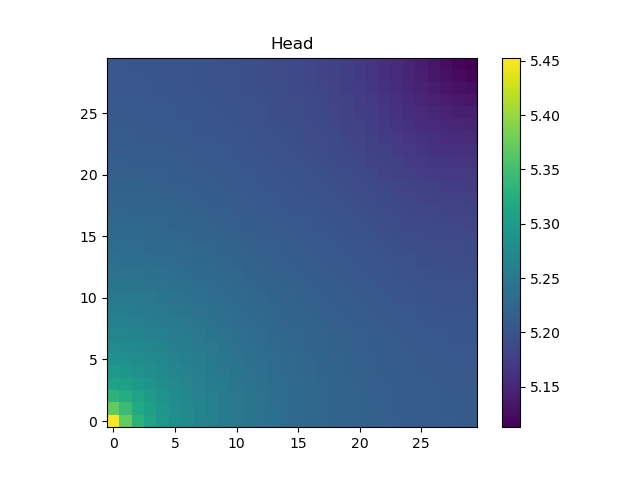
Finally, we can compute the gradient of functions involving the solution of these equations using Zygote.gradient or Zygote.pullback.
hflat2h3d(h) = reshape(h, reverse(ns)...)
gradient_node = div(size(coords, 2) + ns[3] * ns[2], 2)
gradient_node_x = coords[1, gradient_node]
gradient_node_y = coords[2, gradient_node]
grad = Zygote.gradient((x, y)->hflat2h3d(solveforh(x, y)[:, end])[gradient_node], logKs, dirichleths)#calculate the gradient (which involves a redundant calculation of the forward pass)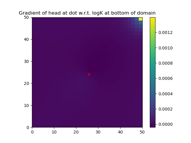
The examples illustrate more advanced usage including inverse problems, combining DPFEHM with a neural network, flow on discrete fracture networks, as well as solving the advection-dispersion and wave equations.
DPFEHM generally uses a two-point flux approximation to discretize the equations. This means, for example, that when the fluid flux between cell
DPFEHM is provided under a BSD style license. See LICENSE.md file for the full text.
This package is part of the Orchard suite, known internally as C20086 Orchard.
If you would like to contribute to DPFEHM, please for the repo and make a pull request. If you have any questions, please contact Daniel O'Malley, omalled@lanl.gov.