- Preprocessing
- Bias and Variance
- Regularization
- Overfitting
- Class Imbalance
- Classifier Types
- Type I and II errors
- Naive Bayes
- Performance Metrics
- Evaluating ML Models
- Improving training/test
- Meta Algorithms
- Decision Trees
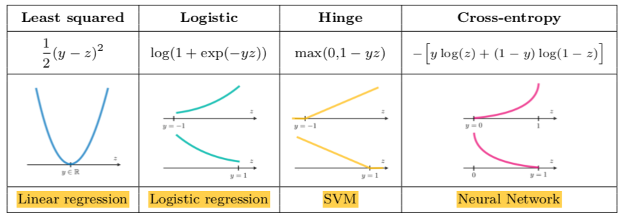
- Loss functions
- Paper
- Tree-based models doesn't depend on scaling
- Non-tree-based models hugely depend on scaling.
- Normalization to [0, 1]
- Standardization to mean=0, std=1
- Remove outliers
bias of an estimator β^ is the difference between its expected value E[β^] and the true value of a parameter β being estimated. More concretely, we compute the prediction bias as the difference between the expected prediction accuracy of our model and the true prediction accuracy. Difference between the expected(or average) prediction of our model and the correct value which we are trying to predict. Higher bias means underfitting and the model we got is simple
The variance is simply the statistical variance of the estimator β^ and its expected value E[β^]
The variance is a measure of the variability of our model’s predictions if we repeat the learning process multiple times with small fluctuations in the training set. Error from sensitivity to small fluctuations in the training set. higher variance means that our model is overfitting and it's a way complex model.
E[(y-fcap)^2] = sigma^2 + Var[fcap] + Bias[fcap]^2 there sigma^2 is the irreducible error
- L2 regularization or Ridge Regression cannot zero out coefficients.
- L1 regularization or Lasso Regression can zero out coefficients(good for sparse data).
- Elastic Net = Best of both worlds. (
lambda * ((j * L1)+((1-j)*L2)) - From Bayes perspective, regularization is to add a prior knowledge to the model. For example, L2 is similar to add a gaussian distribution prior with N(0,1/λ). When λ=0, it means no regularization, then in the other words, we can treat it as covariance is infinite; when λ→inf, then convirance is to zero, then the variance of the parameters in the model is small, consequently, the model is more stable.
- Least absolute deviations is robust in that it is resistant to outliers in the data.
Early Stopping, Data argumentation(numbers of parameter is much smaller than the data ), cross-validation, Regularization (L1, L2), Dropout...
- Get more data
- Generate synthetic data
- Undersampling/Oversampling
- Regularization
Generative classifiers learn a model of the joint probability, p(x, y), of the inputs x and the label y, and make their predictions by using Bayes rules to calculate p(ylx), and then picking the most likely label y. Discriminative classifiers model the posterior p(ylx) directly, or learn a direct map from inputs x to the class labels.
- Type I error is false positive
- Type II error is false negative
What it essentially does it find the posterior probability given the prior. Called Naive because it assumes that X|Y is normally distributed with zero covariance.
- Accuracy sucks as a metric. Misleading.
- Better to use Precision, Recall and ROC curves.
- Precision :
TruePositives/TruePositives+FalsePositives - Specificity:
TrueNegatives/TrueNegatives+FalsePositives - Recall :
TruePositives/TruePositives+FalseNegatives= Sensitivity Precision is the number of positive predictions divided by the total number of positive class values predicted. Recall is the number of positive predictions divided by the number of positive class values in the test data.
- Precision :
- ROC curves: Plot sensitivity vs 1-specificity. ROC stands for Receiver Operating Characteristic.
- F1 Score is
2*((precision*recall)/(precision+recall)). Tells the balance between precision and recall.
print((TP + TN) / float(TP + TN + FP + FN))
When the actual value is positive, how often is the prediction correct? Also known as "True Positive Rate" or "Recall"
sensitivity = TP / float(FN + TP)
When the actual value is negative, how often is the prediction correct?
specificity = TN / (TN + FP)
When the actual value is negative, how often is the prediction incorrect?
false_positive_rate = FP / float(TN + FP)
When a positive value is predicted, how often is the prediction correct?
precision = TP / float(TP + FP)
- Identify if FP or FN is more important to reduce
- Eg : Spam filter: optimize for precision or specificity
- Fraud Detector: optimize for sensitivity
When to use ROC
- insensitive to changes in class distribution (ROC curve does not change if the proportion of positive and negative instances in the test set are varied)
- can identify optimal classification thresholds for tasks with differential misclassification costs
- The AUC value is equivalent to the probability that a randomly chosen positive example i s ranked higher than a randomly chosen negative example. When data sets are imbalanced, ROC/AUC is more stable than Recall, F1, precision. Most binary classifiers give a prediction probability for positive and negative classes. If you set a threshold say, 0.6, you will get a Recall(TPR) and False alarm(FPR). then you vary this threshold value, you will get a group of points. threshold value = 0 corresponds to the point (1,0) while threshold value = 1 corresponds to point(0,0)
When to use PR
- show the fraction of predictions that are false positives
- well suited for tasks with lots of negative instances
Plots sensitivity vs False Positive Rate. The probabilistic interpretation of ROC-AUC score is that if you randomly choose a positive case and a negative case, the probability that the positive case outranks the negative case according to the classifier is given by the AUC
The percentage of the ROC plot that is underneath the curve. AUC is useful as a single number summary of classifier performance
Higher value = better classifier
AUC is useful even when there is high class imbalance (unlike classification accuracy)
- Random resampling
- Stratified resampling
- Cross Validation
Short for Adaptive Boosting, the output of the other learning algorithms ('weak learners') is combined into a weighted sum that represents the final output of the boosted classifier. AdaBoost is adaptive in the sense that subsequent weak learners are tweaked in favor of those instances misclassified by previous classifiers. AdaBoost is sensitive to noisy data and outliers.
- Training set selection: random subset weighted by weight of each data sample
- Classifier output weight: final prediction is a weighted sum of individual weak learners. The weights are definied by the missclassification rate where if accuracy is less than 50 percent then the weight is negative.
Gradient boosting builds an ensemble of trees one-by-one, then the predictions of the individual trees are summed:
D(x) = d_tree1(x) + d_tree2(x) + ...
D(x) + d_tree4(x) = f(x)
R(x) = f(x) - D(x)
- Bagging : Bootstrap AGGregatING uses a variation of data samples to train different base classifiers. Used with unstable classifiers which are sensitive to variations in training set(eg Decision Trees, Perceptrons). Used for reducing variance. Bagging (stands for Bootstrap Aggregation, parallel ensemble) is the way decrease the variance of your prediction by generating additional data for training from your original dataset using combinations with repetitions to produce multisets of the same cardinality/size as your original data(samples are drawn with replacement). By increasing the size of your training set you can't improve the model predictive force, but just decrease the variance and helps to avoid overfitting, narrowly tuning the prediction to expected outcome. If training size is n, build m subsets of size n'(sampling with replacement). if n' = n, then number of unique entries is (1-1/e). This is called bootstrap
- Boosting : Used to convert weak learners to strong ones. Attaches weights proportionate to the amount of misclassification. Primarily used to reduce bias. Boosting(sequential ensemble) is a two-step approach, where one first uses subsets of the original data to produce a series of averagely performing models and then "boosts" their performance by combining them together using a particular cost function (=majority vote). Unlike bagging, in the classical boosting the subset creation is not random and depends upon the performance of the previous models: every new subsets contains the elements that were (likely to be) misclassified by previous models.
- Stacking : Uses an ensemble to extract features which are then again fed into an ensemble. Stacking is a similar to boosting: you also apply several models to your original data. The difference here is, however, that you don't have just an empirical formula for your weight function, rather you introduce a meta-level and use another model/approach to estimate the input together with outputs of every model to estimate the weights or, in other words, to determine what models perform well and what badly given these input data.
-
Non-parametric, supervised learning algorithms
-
Given the training data, a decision tree algorithm divides the feature space into regions. For inference, we first see which region does the test data point fall in, and take the mean label values (regression) or the majority label value (classification).
-
Construction: top-down, chooses a variable to split the data such that the target variables within each region are as homogeneous as possible. Two common metrics: gini impurity or information gain, won't matter much in practice.
-
Advantage: simply to understand & interpret, mirrors human decision making
-
Disadvantage:
- can overfit easily (and generalize poorly)if we don't limit the depth of the tree
- can be non-robust: a small change in the training data can lead to a totally different tree
- instability: sensitive to training set rotation due to its orthogonal decision boundaries https://github.com/ShuaiW/ml-interview#Decision tree
-
gini : g = ((1 – (g1_1^2 + g1_2^2)) * (ng1/n)) + ((1 – (g2_1^2 + g2_2^2)) * (ng2/n)), where g is the gini index for the split point, g1_1 is the proportion of instances in group 1 for class 1, g1_2 for class 2, g2_1 for group 2 and class 1, g2_2 group 2 class 2, ng1 and ng2 are the total number of instances in group 1 and 2 and n are the total number of instances we are trying to group from the parent node.
-
entropy = - p(a)*log(p(a)) - p(b)*log(p(b))
-
Information gain: based towards multivalued attributes.
-
Gain ratio: prefer unbalanced splits in which on partition is much smaller than the other.
-
Gini Index:
- based towards multivalued attributes.
- favor equal-sized partitions
DIVE(Distributional inclusion vector embedding) difference from skipgram
- all word embeddings and context embeddings are contrained to be non negative
- the weights of negative sampling for each word is inversely proportional to its frequency
DIVE was originally designed to perform unsupervised hypernymy task detection and its goal is to preserve the inclusion relation between two context features in the sparse bag of words
- When the co-occured context histogram of y includes that of word x, it means for all context words c in the vocalbulary v, c will co-occur more times with y than x.
- each basis index of DIVE corresponds to a topic and the embedding value at that index represents how often the word appears in the topic