support multiple gain margins #784
Comments
|
@shaikinast Can you add the code that was used to generate the plot? That will help us figure out why you are getting that result. |
|
Sure, please see below the code. Bode diagrams of two almost identical open-loop transfer functions are plotted. The stability margins are printed. In the first case, the gain margin correctly shows Inf, as approved by the Bode diagram. In the second case, the gain margin wrongly shows zero, contrary to the Bode diagram. Your advice is highly appreciated! Thanks, |
|
If you look at the Nyquist plots for the two systems, you can see why you are getting different answers:
Both systems are stable in closed loop, but the first system is open loop unstable and the second system is open loop stable. And the first system is tricky since while it is true that you can multiply the gain by a number greater than 1 and not get any new encirclements, if you multiply the gain by a very small number, the system will eventually lose one encirclement and the closed loop system becomes unstable. If you expand out the range of the Bode plot, you can also see what is going on. Here are the results with
Note that in both systems there is a pole at very low frequency (~1e-17). This example shows one of the challenges in determining the gain margin for a system that is unstable in the open loop: if you make the loop gain small enough, you end up with an unstable system! This type of situation is sometimes called "conditional stability" and is discussed briefly in FBS (just before Section 10.3). It is not really clear what the definition of the gain margin should be for a system that is conditionally stable. In FBS we define gain margin as "the smallest multiplier of the loop gain that makes the system unstable". By that definition, the computation for the first system is correct: if you multiply the loop gain by 0 (the smallest possible loop gain), you get an unstable system! |


|
Another term I have heard used for this is "negative gain margin." Not because the gain is a negative number, but because when converted to decibels, the result is negative (i.e. a number below 1 is a negative number of decibels). It might be worth incorporating the ability to compute negative gain margins, which it looks like is not currently supported in the library. |
|
Matlab offers an example of negative gain margin here: https://www.mathworks.com/help/control/ug/assessing-gain-and-phase-margins.html I'll turn this into an enhancement feature request. |
|
Don't we already support finding margins of conditionally stable systems? |
|
@roryyorke good point. changing the title to indicate support for multiple margins, like |
|
Thank you all for the comments! Some follow-ups:
|
Consider transfer function g(s) = a/(s-1) with a>0. The closed loop TF is h(s) = a/(s-1) / (1 + a/(s-1)) = a / (s-1+a) For stability, we require a-1>0 => a>1. Let a = k * a0, with a0 > 1 and k > 0. System is stable for k*a0 > 1 => k > 1/a0. As a0 tends to infinity, the lower bound on k approaches 0. There's also an intuitive argument: if the system to be controlled is open-loop unstable, then feedback is required for stability; setting the feedback gain to 0 disables feedback, and must make the system unstable. In the above example, as the stabilizing factor a0 gets large, the gain margin k also becomes larger in multiplicative (dB) terms.
Is the system open-loop unstable?
We do have |
|
For the Nyquist plots that I showed, I just used |
Good point. Looks like we do support that already. I'll make sure I have time to check first before I make future changes to this thread. To that end - this sounds like a system in which there is a minimum gain, below which it goes unstable. I think this is the definition of a negative gain margin - how much lower can the gain go before going unstable. Does that sound right? @shaikinast suggests that the library gives this value as something like 1e-16, but I have not gotten around to check if that number is correct. |
|
Conclusion: it might be good to compute margins of SS systems without converting to TF, but in this case the benefit would be negligible; the difference between a gain margin of By adapting @shaikinast 's script, we can see this example suffers from conversion to TF. (Code is at the end.) Here's a Bode plot of the two loop transfer functions as state-space systems; this show's @shaikinast 's intuition that the stability should not have changed is correct:
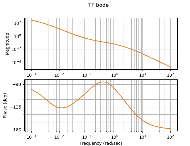
Here are the Bode plots as transfer functions (this is the similar to @murrayrm 's result above, though the frequencies look a bit different; not sure it matters):
The calculated margins between SS and TF are exactly the same; this is because The almost-0 margin of the TF form is due to one pole of the open loop TF being just in the RHP. All the other poles, and all the zeros, are in the LHP plane, so it's not surprising that the merest sliver of gain makes it stable. This is borne out by reducing the gain to nearly zero and checking the closed-loop pole position:
import numpy as np
import control as ct
import matplotlib.pyplot as plt

def par_h():
    par = dict()
    par['P_nom'] = 22e6
    par['P'] = 22e6
    par['Lambda'] = 1.68e-3
    par['beta_i'] = np.array([14.2, 92.4, 78.0, 206.6, 67.1, 21.8]) * 1e-5
    par['lambda_i'] = np.array([0.0127, 0.0317, 0.116, 0.311, 1.40, 3.87])
    par['q'] = 0.96
    par['c_f'] = 977
    par['c_m'] = 1697.0
    par['c_c'] = 5188.6
    par['m_f'] = 2002.0
    par['m_m'] = 11573.0
    par['m_c'] = 500.0
    par['m_dot'] = 17.5
    par['Tf0'] = 1105
    par['Tm0'] = 1087
    par['T_in'] = 864.0
    par['T_out'] = 1106.0
    par['alpha_f'] = -2.875e-5
    par['alpha_m'] = -3.696e-5
    par['beta'] = np.sum(par['beta_i'])
    par['Tc0'] = (par['T_in'] + par['T_out']) / 2.0
    par['Kfm'] = par['q'] * par['P_nom'] / (par['Tf0'] - par['Tm0'])
    par['Kmc'] = par['P_nom'] / (par['Tm0'] - par['Tc0'])

    return par


def sys_h(par, **kwargs):
    par.update(kwargs)
    num_del = len(par['beta_i'])
    nv = num_del + 1

    G0 = dict()
    H = dict()
    sys = dict()
    tf = dict()

    G0['A'] = np.zeros([nv, nv])
    G0['B'] = np.zeros([nv, 1])
    G0['C'] = np.zeros(nv)
    G0['D'] = np.zeros(1)

    G0['A'][0, 0] = -par['beta']/par['Lambda']
    for i in range(1, nv):
        G0['A'][0, i] = par['beta_i'][i-1] / par['Lambda']
        G0['A'][i, 0] = par['lambda_i'][i-1]
        G0['A'][i, i] = -par['lambda_i'][i - 1]
    G0['B'][0] = 1 / par['Lambda']
    G0['C'][0] = 1

    H['A'] = np.zeros([3, 3])
    H['B'] = np.zeros([3, 1])
    H['C'] = dict()
    H['D'] = np.zeros(1)

    H['A'][0, 0] = -par['Kfm'] / (par['m_f'] * par['c_f'])
    H['A'][0, 1] = par['Kfm'] / (par['m_f'] * par['c_f'])
    H['A'][1, 0] = par['Kfm'] / (par['m_m'] * par['c_m'])
    H['A'][1, 1] = -(par['Kfm'] + par['Kmc']) / (par['m_m'] * par['c_m'])
    H['A'][1, 2] = par['Kmc'] / (par['m_m'] * par['c_m'])
    H['A'][2, 1] = par['Kmc'] / (par['m_c'] * par['c_c'])
    H['A'][2, 2] = -(par['Kmc'] + 2 * par['m_dot'] * par['c_c']) / (par['m_c'] * par['c_c'])
    H['B'][0] = par['q'] / (par['m_f'] * par['c_f'])
    H['B'][1] = (1 - par['q']) / (par['m_m'] * par['c_m'])
    H['C']['f'] = np.array([1, 0, 0])
    H['C']['m'] = np.array([0, 1, 0])
    H['C']['c'] = np.array([0, 0, 1])

    sys['G0'] = ct.ss(G0['A'], G0['B'], G0['C'], G0['D'])
    sys['H_f'] = ct.ss(H['A'], H['B'], H['C']['f'], H['D'])
    sys['H_m'] = ct.ss(H['A'], H['B'], H['C']['m'], H['D'])
    sys['H_c'] = ct.ss(H['A'], H['B'], H['C']['c'], H['D'])
    sys['H'] = par['P'] * (par['alpha_f'] * sys['H_f'] +
                           par['alpha_m'] * sys['H_m'])

    # defer TF transformation
    # tf['G0'] = ct.ss2tf(sys['G0'])
    # tf['H'] = ct.ss2tf(sys['H'])
    # tf['G'] = tf['G0'] / (1 - tf['G0'] * tf['H'])

    return sys

par = par_h()
sys_dict1 = sys_h(par)

par['lambda_i'][5] = 5
sys_dict2 = sys_h(par)

l1 = -sys_dict1['G0'] * sys_dict1['H']
l2 = -sys_dict2['G0'] * sys_dict2['H']

print(f'{ct.margin(l1)=}')
print(f'{ct.margin(l2)=}')

ct.bode([l1,l2])
plt.suptitle('SS bode')

## tf
l1_tf = ct.tf(l1)
l2_tf = ct.tf(l2)

# these are identical to above; this calc done on TF?
print(f'{ct.margin(l1_tf)=}')
print(f'{ct.margin(l2_tf)=}')

plt.figure()
ct.bode([l1_tf,l2_tf])
plt.suptitle('TF bode')

## explore stability margin of 0

## this pole is *JUST* in the RHP
print(f'{np.sort((l1_tf.pole().real))[-2:]=}')
## all zeros in the LHP
print(f'{max(l1_tf.zero().real)=}')

ks = np.geomspace(1,1e-10,11)
maxclpole = np.array([max(ct.feedback(k*l1_tf).pole().real)
                      for k in ks])

# check all closed loop stable
assert all(maxclpole < 0)

fig, ax = plt.subplots()
plt.loglog(ks, -maxclpole)
plt.xlabel('gain')
plt.ylabel(r'-max Re $\sigma$')
plt.grid()
plt.title('Stability versus gain')

plt.show() |


|
Thank you @roryyorke for the great explanation! I understand that the problem appears when converting from SS to TF. By the way, do you have any idea why it happens? Also, I understand that |
|
Sorry, I was wrong. I thought I was running python-control 0.9.2, but it was 0.9.1. When I ran the above in 0.9.2, I got the "expected" result:
and
and output: In this case the state-space form of L1 norm happens to have a RHP pole: python-control 0.9.1 and 0.9.2 produce different (but equivalent) state space representations, and these differences, along with round-off error, give rise to these stability differences. I think the difference in the figures above from the previous results is that the open-loop TFs ended up being open-loop stable with 0.9.2, so the Bode plot isn't extended all the way to 1e-14 rad/s. Given the order of the other poles (magnitude 1e-3 to 1), the pole with magnitude 1e-14 is probably "really" an integrator, and if it isn't, on the time-scale of the other poles it might as well be. Numerical round-off means it can be nudged slightly left or right, ending up in the LHP or RHP. This doesn't really matter: it's close enough to 0 to "look like" an integrator. Although the problem in this case wasn't due to switching to TF form, I still I suggest sticking with state-space form as long as possible; multiplied-out transfer functions are not good for high-order systems. Look up Wilkinson's polynomial to see why. |

Hello,
I'm computing stability margins of a system.
The phase margin (PM) is computed correctly, but the gain margin (GM) shows zero (actually it shows 1E-16).
Analyzing the bode plot of the open-loop (OL) transfer function, it clearly shows that the GM should be infinite, since the phase of the
OL never crosses the -180 deg line (it only converges to it asymptotically as omega approaces infinity).
See below the bode plot of the OL, including stability margins.
Any idea why it happens?
Thanks,
-Shai
The text was updated successfully, but these errors were encountered: