This repository contains source code for the following papers:
- "Seamless retrievals of chlorophyll-a from Sentinel-2 (MSI) and Sentinel-3 (OLCI) in inland and coastal waters: A machine-learning approach". N. Pahlevan, et al. (2020). Remote Sensing of Environment. 111604. 10.1016/j.rse.2019.111604.
- "Robust algorithm for estimating total suspended solids (TSS) in inland and nearshore coastal waters". S.V. Balasubramanian, et al. (2020). Remote Sensing of Environment. 111768. 10.1016/j.rse.2020.111768. Code.
- "Hyperspectral retrievals of phytoplankton absorption and chlorophyll-a in inland and nearshore coastal waters". N. Pahlevan, et al. (2021). Remote Sensing of Environment. 112200. 10.1016/j.rse.2020.112200.
- "A Chlorophyll-a Algorithm for Landsat-8 Based on Mixture Density Networks". B. Smith, et al. (2021). Frontiers in Remote Sensing. 623678. 10.3389/frsen.2020.623678.
- "Leveraging multimission satellite data for spatiotemporally coherent cyanoHAB monitoring". K. Fickas, et al. (2023). Frontiers in Remote Sensing. 1157609. 10.3389/frsen.2023.1157609.
The package can be cloned into a directory with:
git clone https://github.com/ryan-edward-oshea/MDN_V2.git
Alternatively, you may use pip to install:
pip install git+https://github.com/ryan-edward-oshea/MDN_V2
The code may then either be used as a library, such as with the following:
from   MDN               import image_estimates, get_sensor_bands, get_tile_data
import numpy             as np
import matplotlib.pyplot as plt
from   matplotlib.colors import LogNorm
plt.rc('text', usetex=True)

def chunk_array(input_list,n):
	for i in range(0,len(input_list),n):
		yield input_list[i:i+n]

#Generate Chl estimates using MDN
sensor      = 'PRISMA' #MSI, OLI, HICO, OLCI,  (or S3A/S3B for chla,tss,cdom,pc)
product     = 'chl,tss,cdom,pc'   #chl #chl,tss,cdom # chl,tss,cdom,pc

kwargs      = {'product'      : product,
               'sat_bands'    : True if product == 'chl,tss,cdom,pc' else False,
               'sensor'       : sensor}

# Select output test
generate_random_estimates = True
plot_output_products      = False

###### Overwrites kwargs for updated PRISMA model ########
if sensor == 'PRISMA':
    min_in_out_val = 1e-6
    kwargs = {
                'allow_missing'   : False,
                'allow_nan_inp'   : False,
                'allow_nan_out'   : True,

                'sensor'          : sensor,
                'removed_dataset' : "South_Africa,Trasimeno",
                'filter_ad_ag'    : False,
                'imputations'     : 5,
                'no_bagging'      : False,
                'plot_loss'       : False,
                'benchmark'       : False,
                'sat_bands'       : False,
                'n_iter'          : 31622,
                'n_mix'           : 5,
                'n_hidden'        : 446,
                'n_layers'        : 5,
                'lr'              : 1e-3,
                'l2'              : 1e-3,
                'epsilon'         : 1e-3,
                'batch'           : 128,
                'use_HICO_aph'    :True,
                'n_rounds'        : 10,
                'product'         : 'aph,chl,tss,pc,ad,ag,cdom',
                'use_gpu'         : False,
                'data_loc'        : "/home/ryanoshea/in_situ_database/Working_in_situ_dataset/Augmented_Gloria_V3_2/",
                'use_ratio'       : True,
                'min_in_out_val'  : min_in_out_val,
                }

    specified_args_wavelengths = {
                'aph_wavelengths' :  get_sensor_bands(kwargs['sensor'] + '-aph'),
                'adag_wavelengths' :  get_sensor_bands(kwargs['sensor'] + '-adag'),
                }


# Generates estimates from random input to test model functionality
if generate_random_estimates:
    random_data = np.random.rand(3, 3, len(get_sensor_bands(sensor+'-sat')) if kwargs['sat_bands'] else len(get_sensor_bands(sensor)))
    products, product_idxs  = image_estimates(random_data, **kwargs)
    print(products, type(products), products.shape)
    print(product_idxs)


# Plots example chl/tss/cdom estimates from Rrs/band
if plot_output_products:
    tile_path  = '/home/ryan/Downloads/acolite.nc'
    bands, Rrs = get_tile_data(tile_path, sensor, allow_neg=False)

    inp_list   = list(chunk_array(Rrs, 10))

    products_list = []
    for i,Rrs_block in enumerate(inp_list):
        	print("Rrs block #:", i, ' of', len(inp_list) )
        	products, slices  = image_estimates(Rrs_block,**kwargs)
        	products_list.append(products)


    products = np.concatenate(products_list,axis=0)
    for product in slices:
        	print("Product: ", product," Slice: ",slices[product]," Output shape:",np.shape(products[:,:,slices[product]]))

    print("Output products shape is:", np.shape(products))
    print("With slices:", slices)
    chla     = products[:,:,slices['chl']]
    TSS      = products[:,:,slices['tss']]
    cdom     = products[:,:,slices['cdom']]
    print(chla,TSS,cdom)

    fig, (ax1, ax2, ax3) = plt.subplots(1, 3)

    chl_im   = ax1.imshow(chla,vmin=1, vmax=100, cmap='jet', aspect='auto',norm=LogNorm())
    TSS_im   = ax2.imshow(TSS,vmin=1, vmax=100, cmap='jet', aspect='auto',norm=LogNorm())
    cdom_im  = ax3.imshow(cdom,vmin=0.01, vmax=1, cmap='jet', aspect='auto',norm=LogNorm())

    ax1.set_title('Chl')
    ax2.set_title('TSS')
    ax3.set_title('CDOM')

    fig.colorbar(chl_im,  ax=ax1)
    fig.colorbar(TSS_im,  ax=ax2)
    fig.colorbar(cdom_im, ax=ax3)

    plt.savefig('PRISMA_processesd_image.png')
    plt.show()
Note: The user-supplied input values should correspond to Rrs (units of 1/sr).
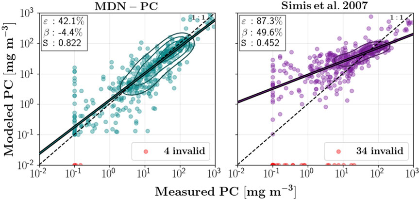
Current performance is shown in the following scatter plots, with 50% of the data used for training and 50% for testing. Note that the models supplied in this repository are trained using 100% of the in situ data, and so observed performance may differ slightly.