/
pw_sc.Rmd
186 lines (155 loc) · 6.87 KB
/
pw_sc.Rmd
1
2
3
4
5
6
7
8
9
10
11
12
13
14
15
16
17
18
19
20
21
22
23
24
25
26
27
28
29
30
31
32
33
34
35
36
37
38
39
40
41
42
43
44
45
46
47
48
49
50
51
52
53
54
55
56
57
58
59
60
61
62
63
64
65
66
67
68
69
70
71
72
73
74
75
76
77
78
79
80
81
82
83
84
85
86
87
88
89
90
91
92
93
94
95
96
97
98
99
100
101
102
103
104
105
106
107
108
109
110
111
112
113
114
115
116
117
118
119
120
121
122
123
124
125
126
127
128
129
130
131
132
133
134
135
136
137
138
139
140
141
142
143
144
145
146
147
148
149
150
151
152
153
154
155
156
157
158
159
160
161
162
163
164
165
166
167
168
169
170
171
172
173
174
175
176
177
178
179
180
181
182
183
184
185
186
---
title: "Pathway activity inference from scRNA-seq"
author:
- name: Pau Badia-i-Mompel
affiliation:
- Heidelberg Universiy
output:
BiocStyle::html_document:
self_contained: true
toc: true
toc_float: true
toc_depth: 3
code_folding: show
package: "`r pkg_ver('decoupleR')`"
vignette: >
%\VignetteIndexEntry{Pathway activity activity inference from scRNA-seq}
%\VignetteEngine{knitr::rmarkdown}
%\VignetteEncoding{UTF-8}
---
```{r setup, include=FALSE}
knitr::opts_chunk$set(
collapse = TRUE,
comment = "#>"
)
```
scRNA-seq yield many molecular readouts that are hard to interpret by
themselves. One way of summarizing this information is by inferring pathway
activities from prior knowledge.
In this notebook we showcase how to use `decoupleR` for pathway activity
inference with a down-sampled PBMCs 10X data-set. The data consists of 160
PBMCs from a Healthy Donor. The original data is freely available from 10x Genomics
[here](https://cf.10xgenomics.com/samples/cell/pbmc3k/pbmc3k_filtered_gene_bc_matrices.tar.gz)
from this [webpage](https://support.10xgenomics.com/single-cell-gene-expression/datasets/1.1.0/pbmc3k).
# Loading packages
First, we need to load the relevant packages, `Seurat` to handle scRNA-seq data
and `decoupleR` to use statistical methods.
```{r "load packages", message = FALSE}
## We load the required packages
library(Seurat)
library(decoupleR)
# Only needed for data handling and plotting
library(dplyr)
library(tibble)
library(tidyr)
library(patchwork)
library(ggplot2)
library(pheatmap)
```
# Loading the data-set
Here we used a down-sampled version of the data used in the `Seurat`
[vignette](https://satijalab.org/seurat/articles/pbmc3k_tutorial.html).
We can open the data like this:
```{r "load data"}
inputs_dir <- system.file("extdata", package = "decoupleR")
data <- readRDS(file.path(inputs_dir, "sc_data.rds"))
```
We can observe that we have different cell types:
```{r "umap", message = FALSE, warning = FALSE}
DimPlot(data, reduction = "umap", label = TRUE, pt.size = 0.5) + NoLegend()
```
### PROGENy model
[PROGENy](https://saezlab.github.io/progeny/) is a comprehensive resource containing a curated collection of pathways and their target genes, with weights for each interaction.
For this example we will use the human weights (other organisms are available) and we will use the top 500 responsive genes ranked by p-value. Here is a brief description of each pathway:
- **Androgen**: involved in the growth and development of the male reproductive organs.
- **EGFR**: regulates growth, survival, migration, apoptosis, proliferation, and differentiation in mammalian cells
- **Estrogen**: promotes the growth and development of the female reproductive organs.
- **Hypoxia**: promotes angiogenesis and metabolic reprogramming when O2 levels are low.
- **JAK-STAT**: involved in immunity, cell division, cell death, and tumor formation.
- **MAPK**: integrates external signals and promotes cell growth and proliferation.
- **NFkB**: regulates immune response, cytokine production and cell survival.
- **p53**: regulates cell cycle, apoptosis, DNA repair and tumor suppression.
- **PI3K**: promotes growth and proliferation.
- **TGFb**: involved in development, homeostasis, and repair of most tissues.
- **TNFa**: mediates haematopoiesis, immune surveillance, tumour regression and protection from infection.
- **Trail**: induces apoptosis.
- **VEGF**: mediates angiogenesis, vascular permeability, and cell migration.
- **WNT**: regulates organ morphogenesis during development and tissue repair.
To access it we can use `decoupleR`:
```{r "progeny", message=FALSE}
net <- get_progeny(organism = 'human', top = 500)
net
```
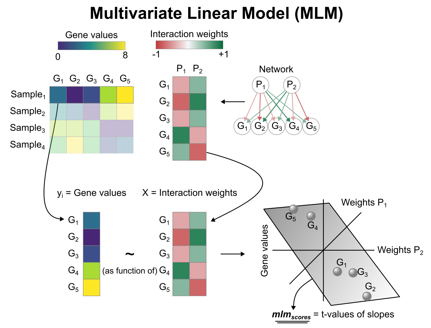
# Activity inference with Multivariate Linear Model (MLM)
To infer pathway enrichment scores we will run the Multivariate Linear Model (`mlm`) method. For each sample in our dataset (`mat`), it fits a linear model that predicts the observed gene expression based on all pathways' Pathway-Gene interactions weights.
Once fitted, the obtained t-values of the slopes are the scores. If it is positive, we interpret that the pathway is active and if it is negative we interpret that it is inactive.
To run `decoupleR` methods, we need an input matrix (`mat`), an input prior
knowledge network/resource (`net`), and the name of the columns of net that we
want to use.
```{r "mlm", message=FALSE}
# Extract the normalized log-transformed counts
mat <- as.matrix(data@assays$RNA@data)
# Run mlm
acts <- run_mlm(mat=mat, net=net, .source='source', .target='target',
.mor='weight', minsize = 5)
acts
```
# Visualization
From the obtained results, we will select the `ulm` activities and store
them in our object as a new assay called `pathwaysmlm`:
```{r "new_assay", message=FALSE}
# Extract mlm and store it in pathwaysmlm in data
data[['pathwaysmlm']] <- acts %>%
pivot_wider(id_cols = 'source', names_from = 'condition',
values_from = 'score') %>%
column_to_rownames('source') %>%
Seurat::CreateAssayObject(.)
# Change assay
DefaultAssay(object = data) <- "pathwaysmlm"
# Scale the data
data <- ScaleData(data)
data@assays$pathwaysmlm@data <- data@assays$pathwaysmlm@scale.data
```
This new assay can be used to plot activities. Here we visualize the Trail
pathway, associated with apoptosis, which seems that in B and NK cells is more
active.
```{r "projected_acts", message = FALSE, warning = FALSE, fig.width = 8, fig.height = 4}
p1 <- DimPlot(data, reduction = "umap", label = TRUE, pt.size = 0.5) +
NoLegend() + ggtitle('Cell types')
p2 <- (FeaturePlot(data, features = c("Trail")) &
scale_colour_gradient2(low = 'blue', mid = 'white', high = 'red')) +
ggtitle('Trail activity')
p1 | p2
```
# Exploration
We can also see what is the mean activity per group across pathways:
```{r "mean_acts", message = FALSE, warning = FALSE}
# Extract activities from object as a long dataframe
df <- t(as.matrix(data@assays$pathwaysmlm@data)) %>%
as.data.frame() %>%
mutate(cluster = Idents(data)) %>%
pivot_longer(cols = -cluster, names_to = "source", values_to = "score") %>%
group_by(cluster, source) %>%
summarise(mean = mean(score))
# Transform to wide matrix
top_acts_mat <- df %>%
pivot_wider(id_cols = 'cluster', names_from = 'source',
values_from = 'mean') %>%
column_to_rownames('cluster') %>%
as.matrix()
# Choose color palette
palette_length = 100
my_color = colorRampPalette(c("Darkblue", "white","red"))(palette_length)
my_breaks <- c(seq(-2, 0, length.out=ceiling(palette_length/2) + 1),
seq(0.05, 2, length.out=floor(palette_length/2)))
# Plot
pheatmap(top_acts_mat, border_color = NA, color=my_color, breaks = my_breaks)
```
In this specific example, we can observe that Trail is more active in B and NK
cells.
# Session information
```{r session_info, echo=FALSE}
options(width = 120)
sessioninfo::session_info()
```