![]()
Simulated annealing (SA) is an algorithm aimed at finding the global minimum of a function E(x0, x1, ..., xn) for a given region ω(x0, x1, ..., xn).
SA relies heavily on sampling random points from the region ω.
In the sections below show how to construct objects of type
SearchSpace.
An interval is a numerical interval defined by a its boundaries. The base class of all intervals is ['Interval'][Interval].
- start: The left boundary of an interval.
- end: The right boundary of an interval.
- continuous interval: An interval that includes start, end, and all points between the boundaries.
- discrete interval: An interval that includes start, end,
as well as a fixed number of points between the boundaries located along an
equidistant grid. To make an interval discrete one has to set the instance
variable
levelsto an integer larger than two. - fixed interval: An interval with numerical boundaries,
see
FixedInterval. - singular interval: A fixed interval that includes a single point, see
SingularInterval. - periodic interval: A fixed interval that wraps around itself. Periodic intervals are useful when defining intervals representing angles e.g. the polar angle of spherical coordinates or the azimuth of cylindrical coordinates.
- parametric interval: An interval with boundaries that depend on other
interval boundaries: see
ParametricInterval.
A search space consists of one or several intervals. A point belonging
to a search space is defined as a list of coordinates.
The class SearchSpace provides methods
for sampling random points from the entire space or
from a region surrounding a given point.
The example below demonstrates how to define a ball shaped 3D
search space using spherical coordinates. The search space includes the
points situated on the spherical surface as well as the inner points.
Note: The function shown below is available as a static function of
the class SearchSpace.
Click to show source code.
import 'dart:math';

import 'package:simulated_annealing/simulated_annealing.dart';

SearchSpace sphere({
    num rMin = 0,
    num rMax = 1,
    num thetaMin = 0,
    num thetaMax = pi,
    num phiMin = 0,
    num phiMax = 2 * pi,
}) {
  // Define intervals.
  final r = FixedInterval(rMin, rMax, name: 'radius <r>');
  final theta = FixedInterval(
    thetaMin,
    thetaMax,
    inverseCdf: InverseCdfs.polarAngle,
    name: 'polar angle <theta>',
  );
  final phi = (phiMin == phiMax)
      ? SingularInterval(phiMin, name: 'azimuth <phi>')
      : PeriodicInterval(phiMin, phiMax, name: 'azimuth <phi>');
  // Defining a spherical search space.
  return SearchSpace.fixed([r, theta, phi],name: 'sphere');
}
The figure below (left) shows 2000 random points generated using the
method next() provided by the class SearchSpace.
The red test point xtest has coordinates [1.9, pi /4, -pi / 2].
The green dots represent points sampled for a
neighbourhood xtest ± deltaPosition around xtest,
where deltaPosition = [0.4, 0.4, ,0.4]
are the perturbation magnitudes along each dimension.
These points were generated using the method perturb().


The figure above (on the right) shows 2000 random points sampled from a
hemispheric search space. The search space includes all points on the
hemisphere obtained by setting rMin = rMax = 2.0 and restricting the
polar angle theta to the range 0...pi/2.
The program used to generate the points is listed in the file [hemispherical_space_example.dart][hemispherical_space_example.dart]. Notice that the perturbation neighbourhood (green dots) does not extend beyond the margins of the search space. If the search space does not intersect the region xtest ± deltaPosition along a certain interval then that respective coordinates is set to NaN.
In the context of simulated annealing, it is advisable to use a search space where each point is equally likely to be chosen. When constructing a search space using intervals the resulting multi-dimensional probability distribution function (PDF) might be non-uniform even if the intervals along each dimension have a uniform PDF.
The examples below aim to demonstrate the problem and its solution.
A simple triangular search space can be defined with the following lines of code:
final gradient = 15.0;
final x = FixedInterval(0, 10);
final y = ParametricInterval(
      () => gradient * x.next(), () => gradient * x.next());
// Defining a spherical search space.
final triangularSpace = SearchSpace([x, y]);
The left figure in the image below shows 2000 points randomly selected from the triangular search space (magenta coloured dots).
There is an aggreggation of points towards the left side of the search space boundary indicating that the 2D PDF of the search_space triangularSpace is non-uniform.
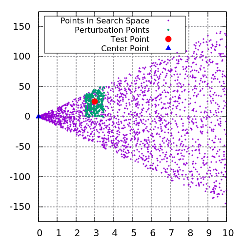
The non-uniform distribution of points along the search space is related to the
uniform distribution of the interval x. For a sufficiently large sample, the number of points with x-coordinate between 0 and 1 is approximately equal to the number of points with x-coordinate between 9 and 10.
However, the size along the vertical dimension of the triangular space decreases linearly from the right to
the left leading to an clustering of points as x approaches 0.
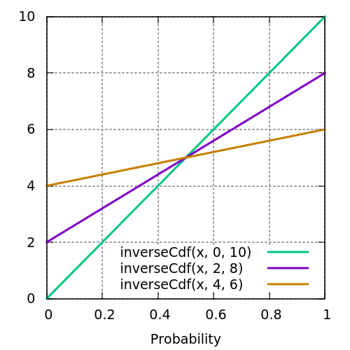
NOTE: When an Interval is constructed without providing an argument for the parameter: inverseCdf, it is implicitly assumed that the values are distributed uniformly between the left and right
interval boundaries and the inverse cummulative distribution function (iCDF) is of the form:
cdf-1(p, xmin, xmax) = xmin + (xmax - xmin)·p where p ∈ [0, 1].
The function iCDF maps a number in the interval [0, 1) to a number in the interval [xmin, xmax).
The graph on the right above shows the implicit iCDF of the interval x for different interval
boundaries.
In order to render the 2D-PDF of the triangular search space uniform we need to provide a suitable iCDF when creating the interval x.
It is clear that the PDF of x must satisfy the conditions: pdf(x < xmin) = 0 and pdf(x > xmax) = 0, since these are the limits of the interval.
Further, assuming that the PDF increases linearly from 0 and is normalized we arrive at:
pdf(x, xmin, xmax) = 2·(x - xmin)/(xmax - xmin)2.
From this it follows that the cummulative distribution function (CDF) defined as cdf(x) = ∫ₓ-∞ pdf(x`) dx` is:
cdf(x, xmin, xmax) = (x - xmin)2/(xmax - xmin)2
and the inverse cummulative distribution function given by:
cdf-1(p, xmin, xmax) = xmin + (xmax - xmin)·√p where p ∈ [0, 1].

The iCDF for the x-coordinate is shown on the right in the image above. It ensures that values of x that are
closer to zero are less likely to be selected.
A triangular space with uniformly distributed points can be instantiated with the following lines of code:
/// The inverse CDF of the interval x.
double inverseCDF(num p, num xMin, num xMax) => xMin + (xMax - xMin) * sqrt(p);
final gradient = 15.0;
final x = FixedInterval(0, 10, inverseCdf: inverseCdf);
final y = ParametricInterval(
() => gradient * x.next(), () => gradient * x.next());
// Defining a spherical search space.
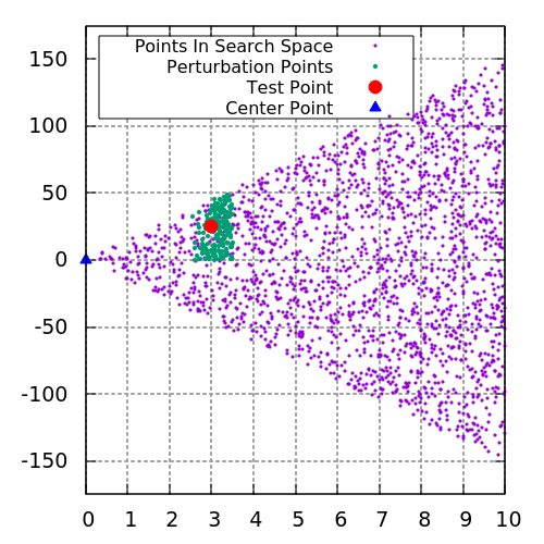
final triangularSpace = SearchSpace([x, y]);The left figure above shows 2000 points randomly selected using the function triangularSpace.next().
It is apparent that the random points are distributed uniformly across the search space.
The first section showed how to use parametric intervals to define a ball shaped search space using Cartesian coordinates. A spherical search space can also be defined in terms of spherical coordinates. In this case, we keep the radius constant and define one interval for the azimuthal angle φ and one for the polar angle θ:
// Define intervals.
final radius = 2;
final phi = FixedInterval(0, 2 * pi);
final theta = FixedInterval(0, pi);
// Defining a spherical search space.
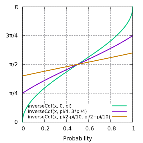
final space = SearchSpace([phi, theta]);The figure below shows 2000 points randomly selected from the search space. It is evident that there is an aggregation of points around the polar areas. The graphs on the right show the iCDF used for the interval θ.


In order to correct the 2-dimensional spherical PDF we have to explicitly specify an iCDF when creating the interval theta. The corrected iCDF of theta takes the form:
cdf-1(p, thetamin, thetamax) = arccos( p · ( cos(thetamin) - cos(thetamax) ) - cos(thetamin) ).
To derive the formula above one starts with the surface area: dA = dφ dθ sin(θ) of the sphere with unity radius to construct the PDF then the CDF and finally the iCDF.
The spherical search space can be constructed with the following lines of code:
double inverseCdf(num p, num thetaMin, num thetaMax) {
  final cosThetaMin = cos(thetaMin);
  return acos(-p * (cosThetaMin - cos(thetaMax)) + cosThetaMin);
}
// Define intervals.
final radius = 2;
final phi = FixedInterval(0, 2 * pi, inverseCdf: inverseCdf);
final theta = FixedInterval(0, pi);

// Defining a spherical search space.
final space = SearchSpace([phi, theta]);
The figure below shows 2000 points randomly selected from the search space with a uniform 2D PDF. The graphs on the right shows a plot of the iCDF for different boundaries thetamin and thetamax.

Please file feature requests and bugs at the issue tracker.