![]()


While many awesome packages for network analysis exist for R, all with their own offerings and advantages, they also all have their own vocabulary, syntax, and expected formats for data inputs and analytic outputs. Many of these packages only work on some types of networks (usually one-mode, simple, directed or undirected networks) for some types of analysis; if you want to analyse a different type of network or try a different analysis, a different package is needed. And they can rely on a very different visual language (and sometimes plotting engine), which can mess up your pretty presentation or paper. This can make learning and using network analysis tools in R challenging.
By contrast, we build packages that offer many analytic tools that
work on many (if not most) types of networks of all kinds. {manynet}
is the first package that helps researchers with Making, Modifying, and
Mapping networks. For Measures, Memberships, or Models, see
{migraph}.
Networks can come from many sources and be found in many different
formats: some can be found in this or other packages, some can be
created or generated using functions in this package, and others can be
downloaded from the internet and imported from your file system.
{manynet} provides tools to make networks from all these sources in
any number of common formats.
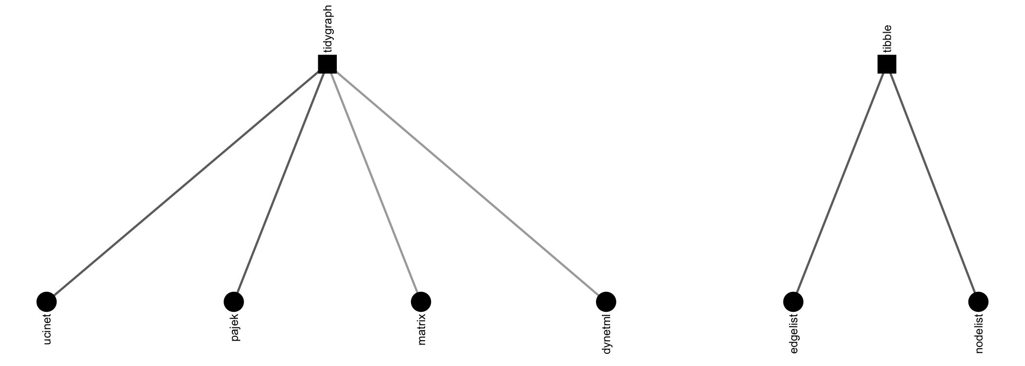
{manynet} offers a number of options for importing network data found
in other repositories. Besides importing and exporting to Excel
edgelists, nodelists, and (bi)adjacency matrices, there are specific
routines included for
UCINET,
Pajek,
GraphML, and
DynetML files, e.g.:
If you cannot remember the file name/path, then just run read_*() with
the parentheses empty, and a file selection popup will open so that you
can browse through your file system to find the file. Usually both
read_*() and write_*() are offered to make sure that {manynet} is
compatible with your larger project and analytic workflow.
read_dynetml(),read_edgelist(),read_graphml(),read_matrix(),read_nodelist(),read_pajek(),read_ucinet()write_edgelist(),write_graphml(),write_matrix(),write_nodelist(),write_pajek(),write_ucinet()
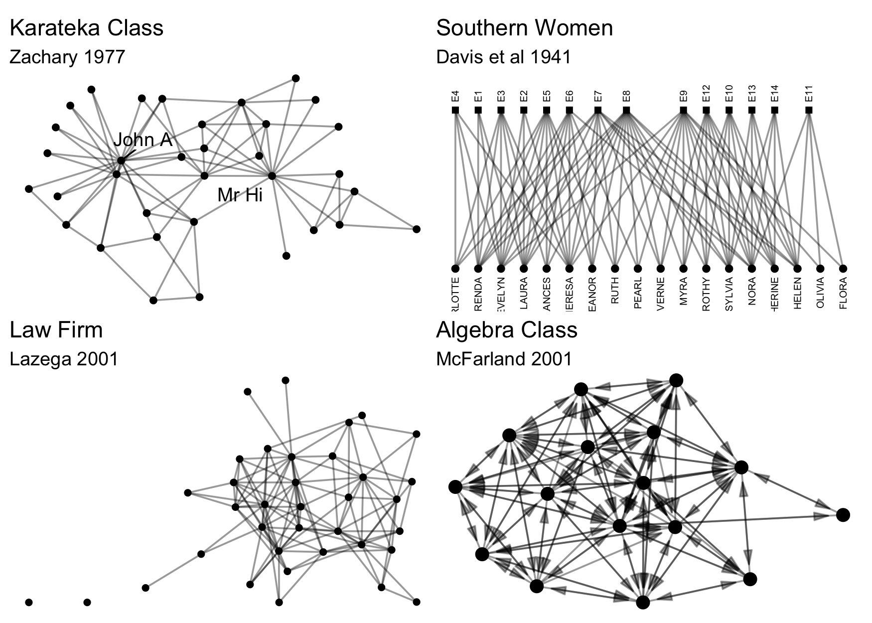
There may be no need to import network data though, if that network data
already exists in a package in R. To facilitate testing and to
contribute to an ecosystem of easily accessible network data,
particularly for pedagogical purposes, we include a number of classical
and instructional network datasets, all thoroughly documented and ready
for analysis. Here are just a few examples, all available in
{manynet}:
Here are some others: ison_adolescents, ison_algebra,
ison_brandes, ison_friends, ison_hightech, ison_karateka,
ison_koenigsberg, ison_laterals, ison_lawfirm, ison_lotr,
ison_marvel_relationships, ison_marvel_teams,
ison_monastery_esteem, ison_monastery_influence,
ison_monastery_like, ison_monastery_praise, ison_networkers,
ison_physicians, ison_potter, ison_southern_women,
ison_starwars, ison_usstates
{manynet} includes functions for making networks algorithmically. The
create_* group of functions create networks with a particular
structure, and will always create the same format from the same inputs,
e.g.:
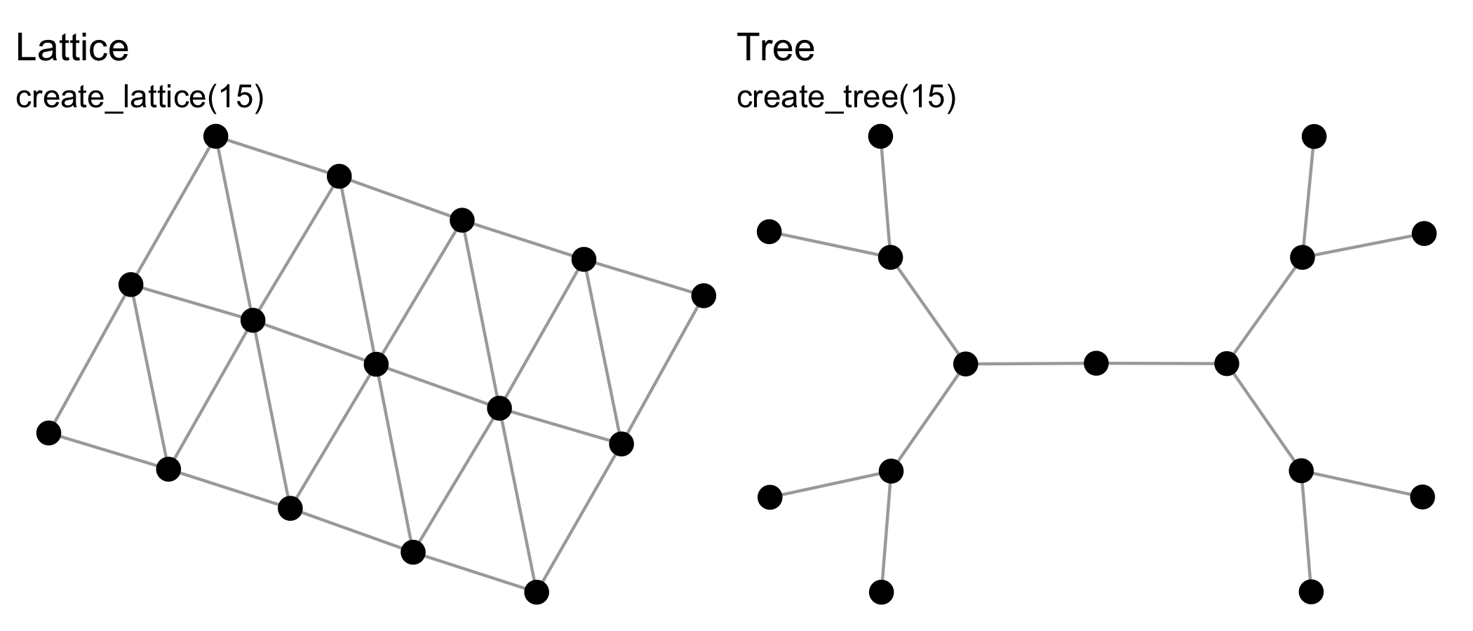
See also create_components(), create_core(), create_empty(),
create_explicit(), create_filled(), create_lattice(),
create_ring(), create_star(), create_tree().
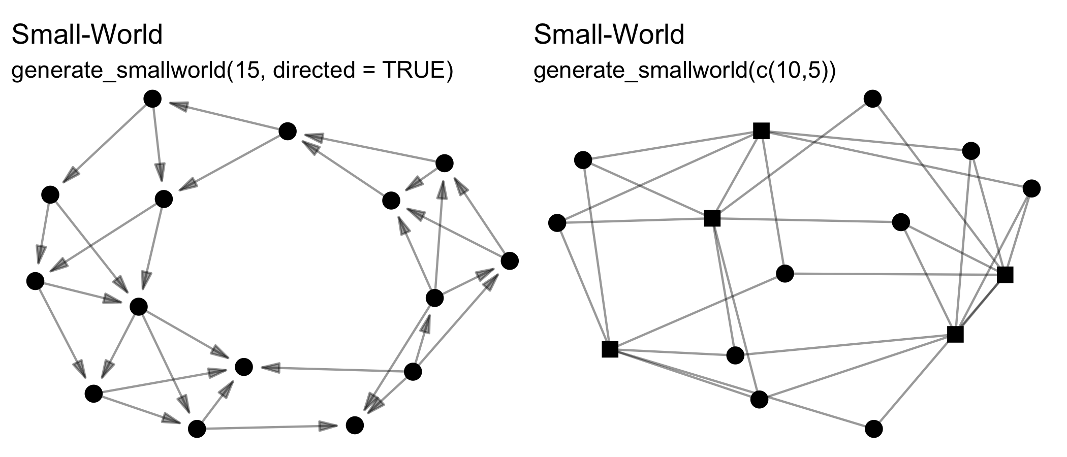
The generate_* group of functions generate networks from generative
mechanisms that may include some random aspect, and so will return a
different output each time they are run, e.g.:
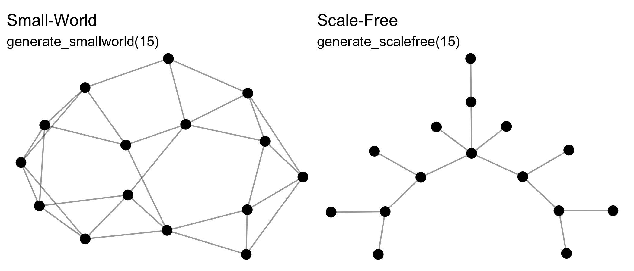
See also generate_permutation(), generate_random(),
generate_scalefree(), generate_smallworld(), generate_utilities().
Note that all these functions can create directed or undirected,
one-mode or two-mode networks. Creating two-mode networks is as easy as
passing the first argument (n) a vector of two integers instead of
one. For example, while n = 15 will create a one-mode network of 10
nodes, whereas n = c(10,5) will create a two-mode network of 10 nodes
in the first mode, and 5 nodes in the second mode. Some of these
functions wrap existing algorithms in other packages, while others are
unique offerings or add additional formats, e.g. two-mode networks.
Lastly, {manynet} also includes functions for simulating diffusion or
learning processes over a given network:
play_diffusion(),play_diffusions(),play_learning(),play_segregation()
The diffusion models include not only SI and threshold models, but also SIS, SIR, SIRS, SEIR, and SEIRS.
Before or during analysis, you may need to modify the network you are
analysing in various ways. Different packages have different syntaxes
and vocabulary for such actions; {manynet}’s to_*() functions can be
used on any class object to reformat, transform, or split networks into
networks with other properties.
Once you have imported network data, identified network data in this or
other packages in R, or invented your own, you may need to translate
this data into another class for analysis. {manynet}’s as_*()
functions can be used to coerce objects from one of many common classes
into any other. Below is a directed graph showing the currently
available options:
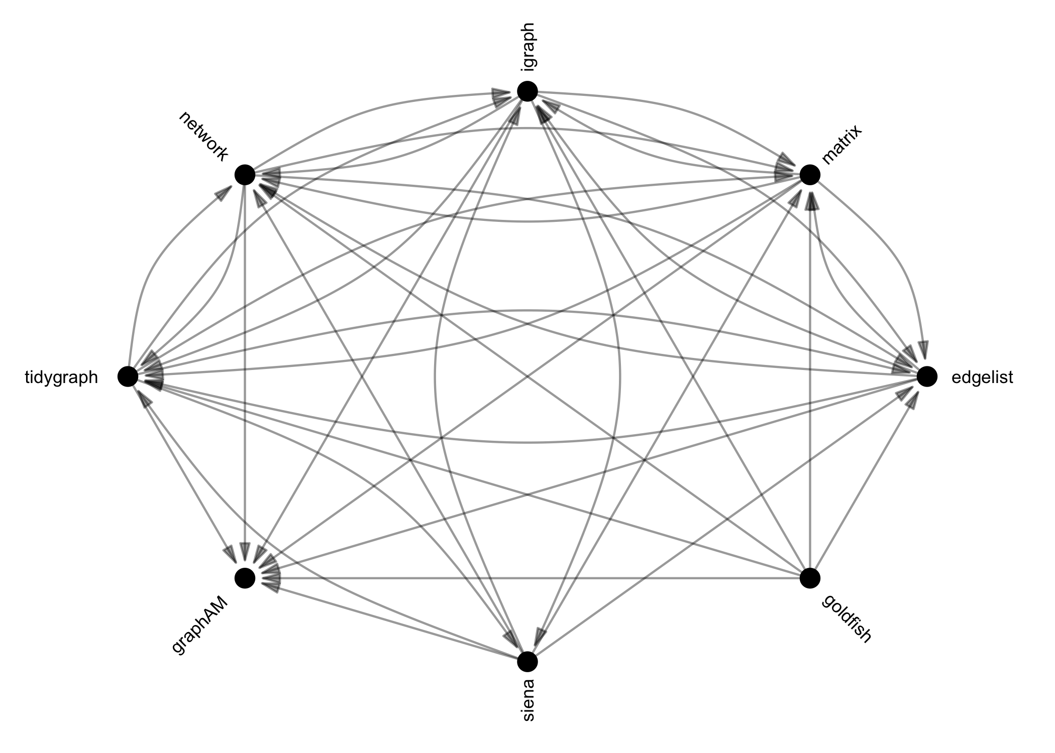
These functions are designed to be as intuitive and lossless as possible, outperforming many other class-coercion packages.
We use these functions internally in every {manynet} and {migraph}
function to (1) allow them to be run on any compatible network format
and (2) use the most efficient algorithm available. This makes
{manynet} and {migraph} compatible with your existing workflow,
whether you use base R matrices or edgelists as data frames,
{igraph}, {network},
or {tidygraph}, and
extensible by developments in those other packages too.
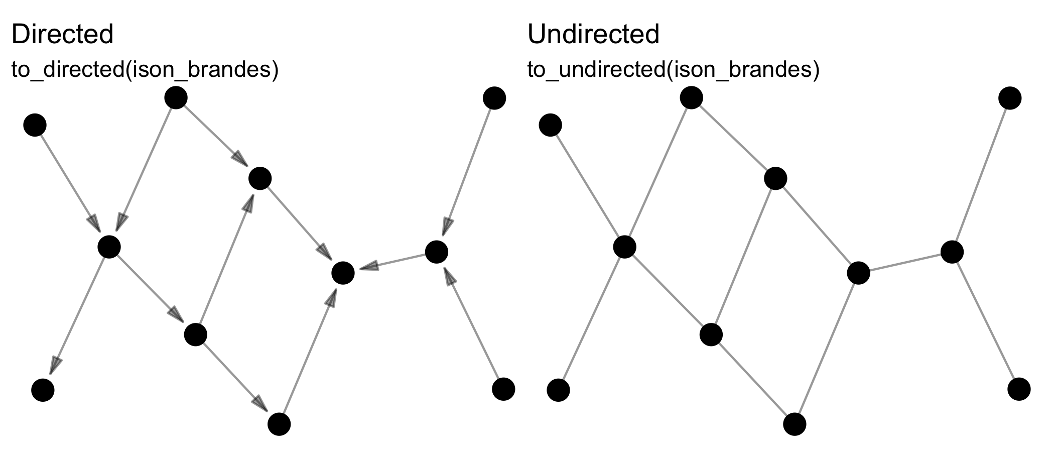
Reformatting means changing the format of the network, e.g. from
directed to undirected via to_undirected().
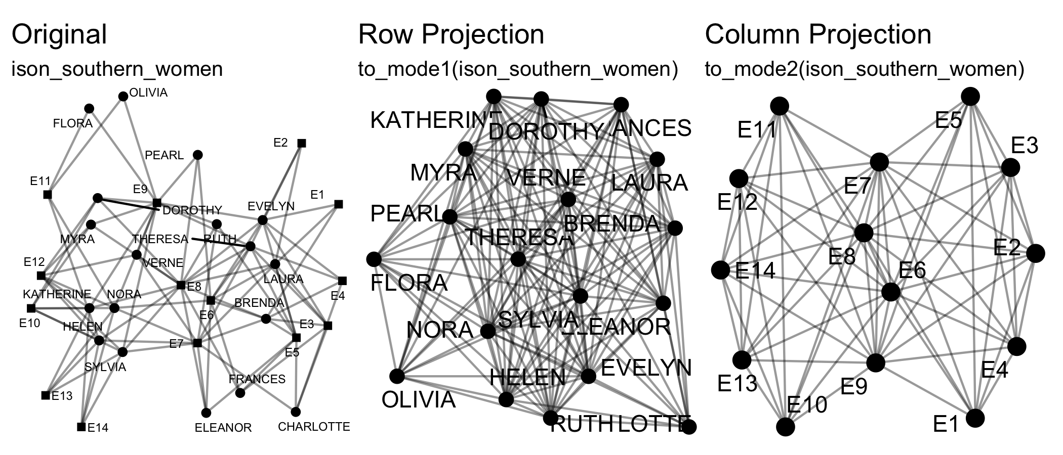
Transforming means changing the dimensions of the network, e.g. from a
two-mode network to a one-mode projection via to_mode1().
Splitting means separating a network, e.g. from a whole network to the
various ego networks via to_egos().
Those functions that split a network into a list of networks are
distinguishable as those to_*() functions that are named in the
plural. Split data can be rejoined using the from_*() family of
functions.
See also to_acyclic(), to_anti(), to_blocks(), to_components(),
to_directed(), to_egos(), to_eulerian(), to_galois(),
to_giant(), to_matching(), to_mentoring(), to_mode1(),
to_mode2(), to_multilevel(), to_named(), to_no_isolates(),
to_onemode(), to_reciprocated(), to_redirected(), to_simplex(),
to_slices(), to_subgraph(), to_subgraphs(), to_ties(),
to_tree(), to_twomode(), to_undirected(), to_uniplex(),
to_unnamed(), to_unsigned(), to_unweighted(), to_waves() and
from_egos(), from_slices(), from_subgraphs(), from_ties(),
from_waves().
{manynet}’s *is_*() functions offer fast logical tests of various
properties. Whereas is_*() returns a single logical value for the
network, node_is_*() returns a logical vector the length of the number
of nodes in the network, and tie_is_*() returns a logical vector the
length of the number of ties in the network.
is_acyclic(),is_aperiodic(),is_complex(),is_connected(),is_directed(),is_dynamic(),is_edgelist(),is_eulerian(),is_graph(),is_igraph(),is_labelled(),is_list(),is_longitudinal(),is_manynet(),is_multiplex(),is_perfect_matching(),is_signed(),is_twomode(),is_uniplex(),is_weighted()node_is_core(),node_is_cutpoint(),node_is_exposed(),node_is_fold(),node_is_infected(),node_is_isolate(),node_is_latent(),node_is_max(),node_is_mentor(),node_is_min(),node_is_random(),node_is_recovered()tie_is_bridge(),tie_is_feedback(),tie_is_loop(),tie_is_max(),tie_is_min(),tie_is_multiple(),tie_is_random(),tie_is_reciprocated()
The *is_max() and *is_min() functions are used to identify the
maximum or minimum, respectively, node or tie according to some measure
(see below).
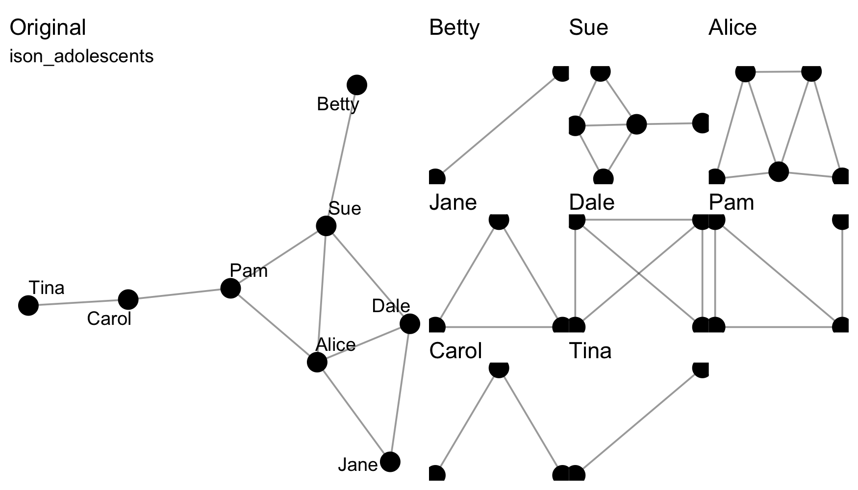
{manynet} includes three one-line graphing functions with sensible
defaults based on the network’s properties.
First, autographr() is used to graph networks in any of the
{manynet} formats. It includes sensible defaults so that researchers
can view their network’s structure or distribution quickly with a
minimum of fuss. Compare the output from {manynet} with a similar
default from {igraph}:
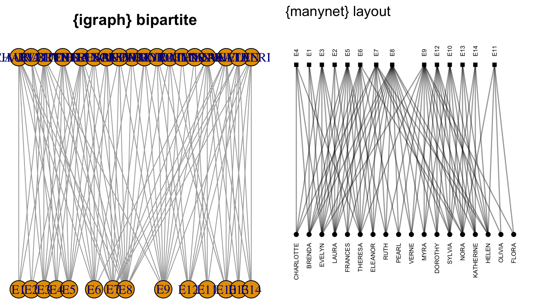
Here the {manynet} function recognises that the network is a two-mode
network and uses a bipartite layout by default, and recognises that the
network contains names for the nodes and prints them vertically so that
they are legible in this layout. Other ‘clever’ features include
automatic node sizing and more. By contrast, {igraph} requires the
bipartite layout to be specified, has cumbersome node size defaults for
all but the smallest graphs, and labels also very often need resizing
and adjustment to avoid overlap. All of {manynet}’s adjustments can be
overridden, however…
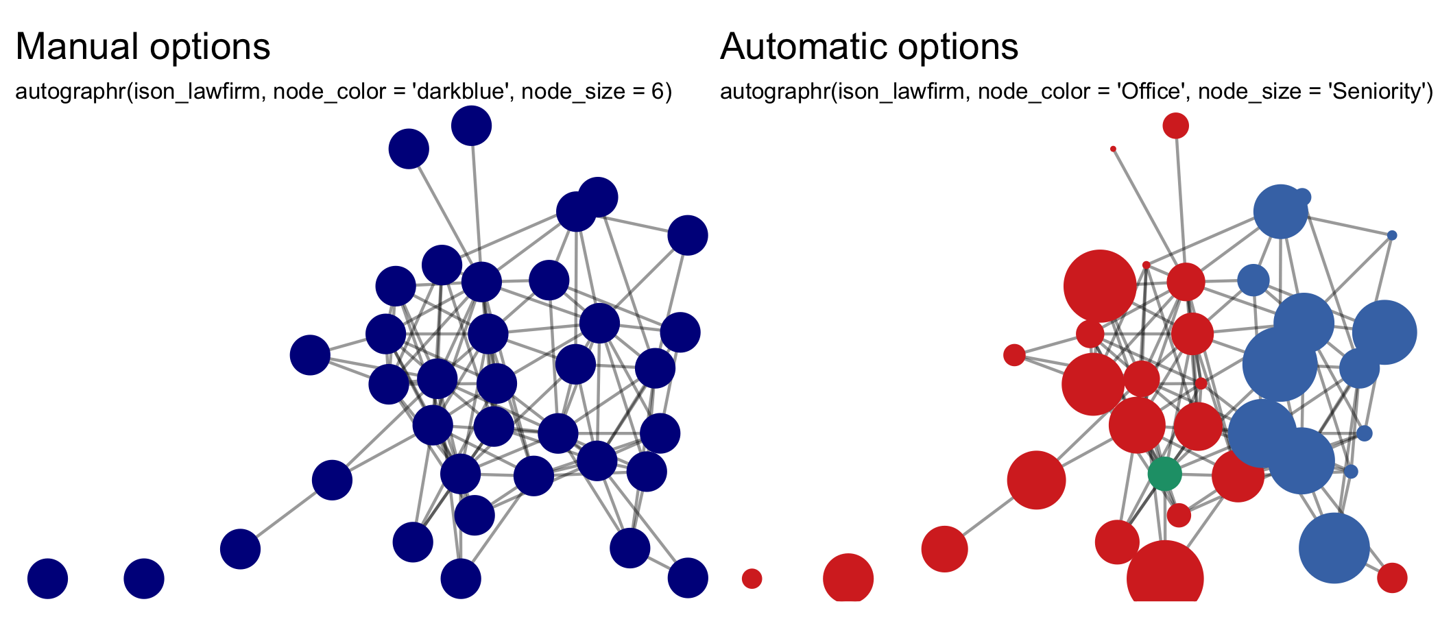
Changing the size and colors of nodes and ties is as easy as specifying the function’s relevant argument with a replacement, or indicating from which attribute it should inherit this information.
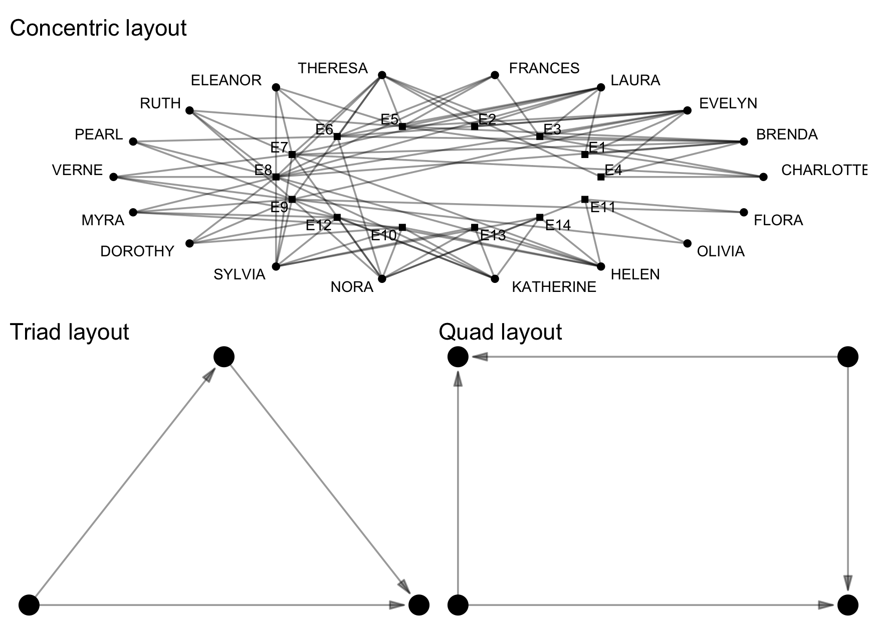
{manynet} can use all the layout algorithms offered by packages such
as {igraph}, {ggraph}, and {graphlayouts}, and offers some
additional layout algorithms for snapping layouts to a grid, visualising
partitions horizontally, vertically, or concentrically, or conforming to
configurational coordinates.
Lastly, autographr() is highly extensible in terms of the overall look
of your plots. {manynet} uses the excellent {ggraph} package (and
thus {ggplot2}) as a plotting engine. This enables alterations such as
the application of themes to be applied upon the defaults. If you want
to quickly make sure your plots conform to your institution or taste,
then it is easy to do with themes and scales that update the basic look
and color palette used in your plots.
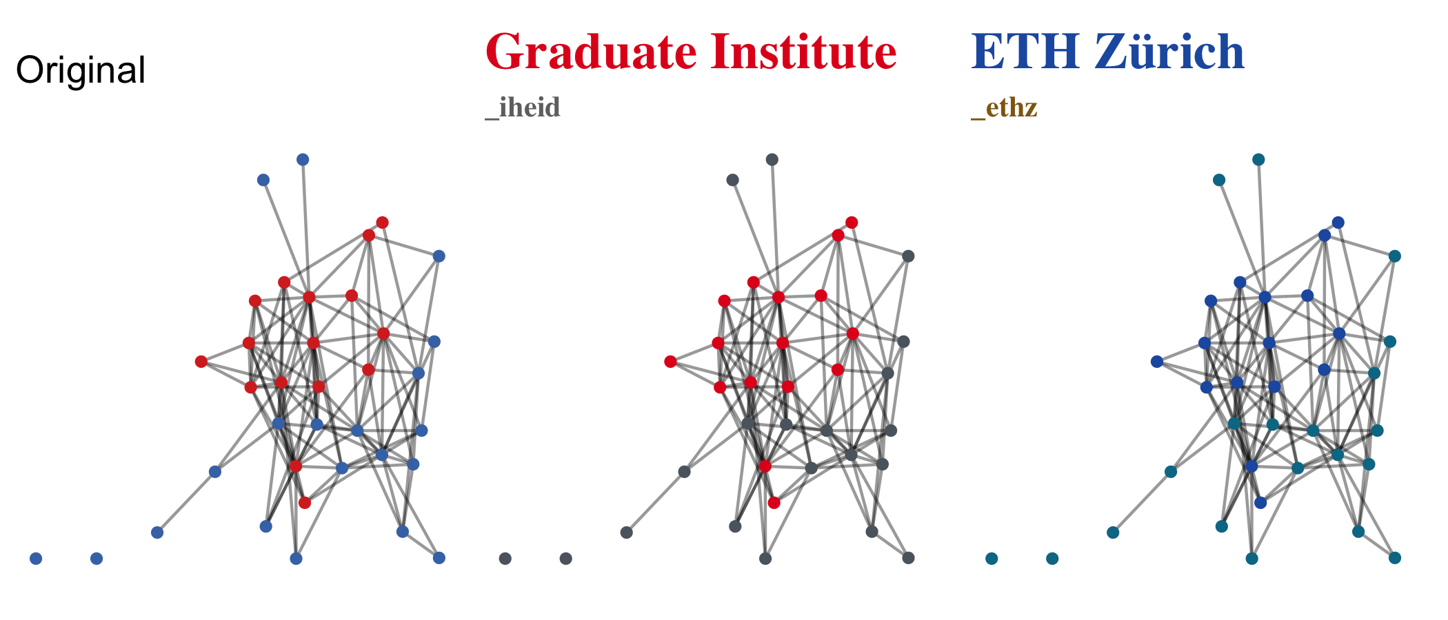
More themes are on their way, and we’re happy to take suggestions.
Second, autographs() is used to graph multiple networks together,
which can be useful for ego networks or network panels. {patchwork} is
used to help arrange individual plots together.
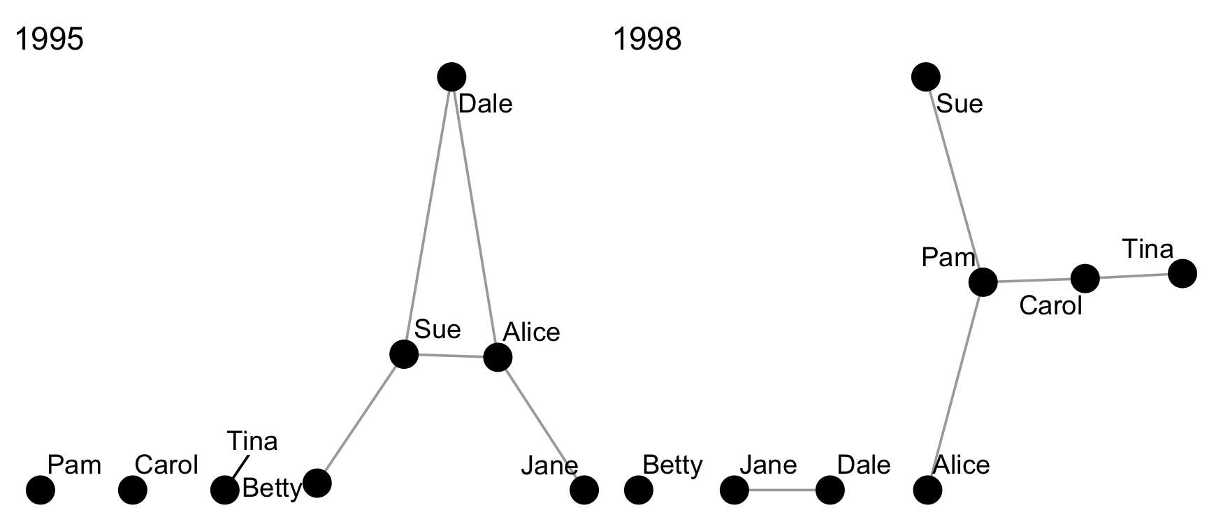
Third, autographd() is used to visualise dynamic networks. It uses
{gganimate} and {gifski} to create a gif that visualises network
changes over time. It really couldn’t be easier.
The easiest way to install the latest stable version of {manynet} is
via CRAN. Simply open the R console and enter:1
install.packages('manynet')
library(manynet) will then load the package and make the data and
tutorials (see below) contained within the package available.
For the latest development version, for slightly earlier access to new features or for testing, you may wish to download and install the binaries from Github or install from source locally. The latest binary releases for all major OSes – Windows, Mac, and Linux – can be found here. Download the appropriate binary for your operating system, and install using an adapted version of the following commands:
- For Windows:
install.packages("~/Downloads/manynet_winOS.zip", repos = NULL) - For Mac:
install.packages("~/Downloads/manynet_macOS.tgz", repos = NULL) - For Unix:
install.packages("~/Downloads/manynet_linuxOS.tar.gz", repos = NULL)
To install from source the latest main version of {manynet} from
Github, please install the {remotes} package from CRAN and then:
- For latest stable version:
remotes::install_github("stocnet/manynet") - For latest development version:
remotes::install_github("stocnet/manynet@develop")
This package includes tutorials to help new and experienced users learn
how they can conduct social network analysis using the package. These
tutorials leverage the additional package {learnr} (see
here), but we have made it easy to
use {manynet} or {migraph} tutorials right out of the box:
run_tute()
#> # A tibble: 8 × 3
#>   package name      title
#>   <chr>   <chr>     <chr>
#> 1 manynet tutorial0 Intro to R
#> 2 manynet tutorial1 Data
#> 3 manynet tutorial2 Visualisation
#> 4 migraph tutorial4 Centrality
#> 5 migraph tutorial5 Community
#> 6 migraph tutorial6 Position
#> 7 migraph tutorial7 Topology
#> 8 migraph tutorial8 Regression
# run_tute("tutorial1")This package stands on the shoulders of several incredible packages.
In terms of the objects it works with, this package aims to provide an
updated, more comprehensive replacement for {intergraph}. As such it
works with objects in {igraph} and {network} formats, but also
equally well with base matrices and edgelists (data frames), and formats
from several other packages.
The user interface is inspired in some ways by Thomas Lin Pedersen’s
excellent {tidygraph} package, though makes some different decisions,
and uses the quickest {igraph} or {network} routines where
available.
{manynet} has inherited most of its core functionality from its
maternal package, {migraph}. {migraph} continues to offer more
analytic and modelling functions that builds upon the architecture
provided by {manynet}. For more, please check out {migraph}
directly.
Development on this package has been funded by the Swiss National Science Foundation (SNSF) Grant Number 188976: “Power and Networks and the Rate of Change in Institutional Complexes” (PANARCHIC).
Footnotes
-
Macs with Macports installed may also install from the command line using Macports. ↩