dsolve returns incorrect result for a first order non-linear ODE

[PopeOfChiliTown]

Input equation:

import sympy as sym
v = sym.Function(v)
t = sym.Symbol('t', real=True, positive=True
g = sym.Symbol('g', real=True, positive=True
D = sym.Symbol('D', real=True, positive=True

diffeq = v(t).diff(t) + g - D*((v(t)**2)
x = sym.dsolve(diffeq, v(t))

Output expression:
Eq(v(t), sqrt(g)/( sqrt(D)*tanh( sqrt(D)*sqrt(g)*(C1-t))))

However, the correct answer to this should have
tanh(sqrt(D)*sqrt(g)*(C1+t)
in the numerator. So the correct output should be something like:
Eq(v(t), (sqrt(g)*(tanh(sqrt(D)*sqrt(g)*(C1+t)) / sqrt(D)

This appears to be a regression as the textbook "Elementary Mechanics using Python" uses an older version of sympy on page 71 and it returns the correct answer. The analytic solution solving the diffeq and showing tanh is in the numerator is on page 70. This book is currently free from springer (https://link.springer.com/book/10.1007/978-3-319-19596-4)

The solution with tanh in the numerator was also verified using mathematica.

[PopeOfChiliTown]

Also verified that the returned solution doesn't satisfy the diffeq:
x.rhs.diff(t) + g - D*(x.rhs**2)

is not equal to zero.

[oscarbenjamin]

The code shown is missing brackets. I had to add those in to test this:

In [16]: t, g, D = symbols('t, g, D', real=True, positive=True)                                                                   

In [17]: eq = v(t).diff(t) + g - D*v(t)**2                                                                                        

In [18]: sol = dsolve(eq, v(t))                                                                                                   

In [19]: sol                                                                                                                      
Out[19]: 
                  √g          
v(t) = ───────────────────────
       √D⋅tanh(√D⋅√g⋅(C₁ - t))

Okay so that's not what you were expecting. It is however a solution of the ODE:

In [20]: checkodesol(eq, sol)                                                                                                     
Out[20]: (True, 0)

In [21]: sol.rhs.diff(t) + g - D*(sol.rhs**2)                                                                                     
Out[21]: 
  ⎛        2                ⎞                            
g⋅⎝1 - tanh (√D⋅√g⋅(C₁ - t))⎠                 g          
───────────────────────────── + g - ─────────────────────
        2                               2                
    tanh (√D⋅√g⋅(C₁ - t))           tanh (√D⋅√g⋅(C₁ - t))

In [22]: simplify(_)                                                                                                              
Out[22]: 0

This form of the solution means that the constant is imaginary:

In [78]: C1 = Symbol('C1')                                                                                                        

In [68]: sol.subs(t, 0).subs(v(0), 0)                                                                                             
Out[68]: 
            √g       
0 = ─────────────────
    √D⋅tanh(C₁⋅√D⋅√g)

In [69]: solve(sol.subs(t, 0).subs(v(0), 0), C1)                                                                                  
Out[69]: 
⎡ -ⅈ⋅π      ⅈ⋅π  ⎤
⎢───────, ───────⎥
⎣2⋅√D⋅√g  2⋅√D⋅√g⎦

Substituting the constant and simplifying gives the expected result (same for either choice of constant):

In [70]: C11, C12 = solve(sol.subs(t, 0).subs(v(0), 0), C1)  

In [73]: sol.subs(C1, C11).simplify()                                                                                             
Out[73]: 
       -√g⋅tanh(√D⋅√g⋅t) 
v(t) = ──────────────────
               √D        

In [74]: sol.subs(C1, C12).simplify()                                                                                             
Out[74]: 
       -√g⋅tanh(√D⋅√g⋅t) 
v(t) = ──────────────────
               √D 

So I think everything is working fine apart from using dsolve with ics directly:

In [77]: dsolve(eq, ics={v(0): 0})                                                                                                
---------------------------------------------------------------------------
NotImplementedError                       Traceback (most recent call last)
<ipython-input-77-719c6d816cc5> in <module>
----> 1 dsolve(eq, ics={v(0): 0})

~/current/sympy/sympy/sympy/solvers/ode/ode.py in dsolve(eq, func, hint, simplify, ics, xi, eta, x0, n, **kwargs)
    651             # The key 'hint' stores the hint needed to be solved for.
    652             hint = hints['hint']
--> 653             return _helper_simplify(eq, hint, hints, simplify, ics=ics)
    654 
    655 def _helper_simplify(eq, hint, match, simplify=True, ics=None, **kwargs):

~/current/sympy/sympy/sympy/solvers/ode/ode.py in _helper_simplify(eq, hint, match, simplify, ics, **kwargs)
    705     if ics and not 'power_series' in hint:
    706         if isinstance(rv, (Expr, Eq)):
--> 707             solved_constants = solve_ics([rv], [r['func']], cons(rv), ics)
    708             rv = rv.subs(solved_constants)
    709         else:

~/current/sympy/sympy/sympy/solvers/ode/ode.py in solve_ics(sols, funcs, constants, ics)
    819 
    820     if len(solved_constants) > 1:
--> 821         raise NotImplementedError("Initial conditions produced too many solutions for constants")
    822 
    823     return solved_constants[0]

NotImplementedError: Initial conditions produced too many solutions for constants

[RituRajSingh878]

@oscarbenjamin why it is returning NotImplementedError? Also, in this case, we can return all values of arbitrary constant.

[oscarbenjamin]

That's correct. The initial condition handling code needs to be improved to give solutions for all values of the constant.

[RituRajSingh878]

Any particular reason for not returning all solutions?

On of the test case says for returning one of the solutions instead of raising.
So any reason for not returning all solutions-

sympy/sympy/solvers/ode/tests/test_ode.py

Lines 100 to 104 in 5db74b0

	def test_dsolve_ics():
	# Maybe this should just use one of the solutions instead of raising...
	with raises(NotImplementedError):
	dsolve(f(x).diff(x) - sqrt(f(x)), ics={f(1):1})

[oscarbenjamin]

Any particular reason for not returning all solutions?

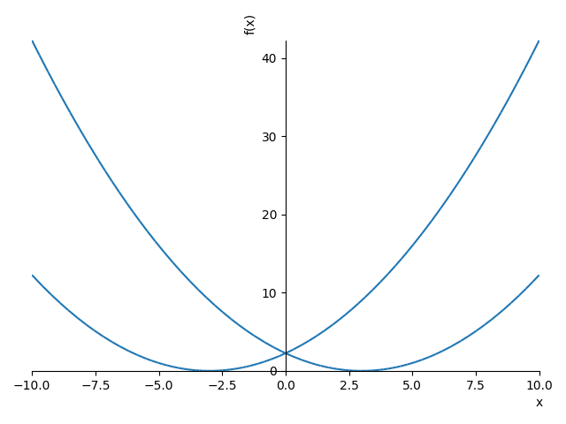
There can be a reason for not returning all solutions. Some methods in particular separation of variables can lead to multiple solutions where some do not in fact satisfy the original ODE. Let's do it manually.

We'll assume that x and t are real although dsolve should not always
assume that.

(1)   dx/dt = sqrt(x)
(2)   \int dx/sqrt(x) = \int dt
(3)   2 sqrt(x) = t - t0
(4)   x = (t - t0)**2 / 4

We can see that the solution curves in the x, t plane are parabolas that look like y=x^2 except shifted left or right e.g. like this:

In [54]: sol = dsolve(x(t).diff(t) + sqrt(x(t)))                                                                                  

In [55]: C1 = Symbol('C1')                                                                                                        

In [60]: p1 = plot(sol.rhs.subs(C1, -3), show=False)                                                                              

In [61]: p2 = plot(sol.rhs.subs(C1, +3), show=False)                                                                              

In [62]: p1.append(p2[0])                                                                                                         

In [63]: p1.show()  

We see here that our two different solution curves intersect which clearly violates the uniqueness of the initial value problem (IVP). The two example curves have the same value at t=0 meaning that an initial condition there might seem consistent with either curve.

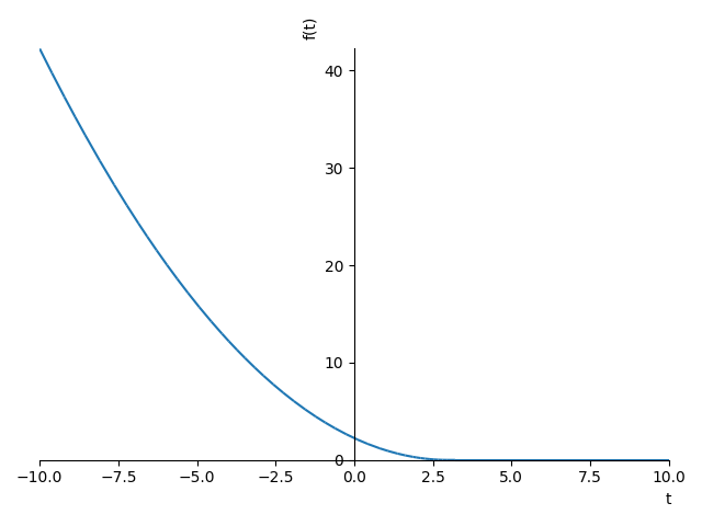
But an IVP should normally have a unique solution. Looking more carefully these solution curves are not everywhere valid. The ODE is dx/dt = - sqrt(x) so this is only sensibly defined if x >= 0 (hence our curves don't exist in the bottom half of the x, t plane). But if x >= 0 then the rhs (-sqrt(x)) should always be nonpositive. That means that the part of the curve that has positive gradient does not satisfy the ODE.

Where did we go wrong? We divided by sqrt(x) which is zero when x is zero. We need to also consider the case that x=0 which is a solution of the ODE as you can easily check. The correct solution here for an inital condition is that we take the curve with negative gradient at that point in the x, t plane and continue it until x=0 after which the solution is just x=0 for all t. That looks like this:

In [82]: sol_full = Piecewise((sol.rhs.subs(C1, -3), t < 3), (0, True))                                                           

In [83]: sol_full                                                                                                                 
Out[83]: 
⎧ 2                     
⎪t    3⋅t   9           
⎪── - ─── + ─  for t < 3
⎨4     2    4           
⎪                       
⎪     0        otherwise
⎩                       

In [84]: plot(sol_full)                                                                                                           
Out[84]: <sympy.plotting.plot.Plot at 0x116479cd0>

This is now a unique solution that satisfies the ODE everywhere.

Why don't the normal uniqueness conditions for ODEs work here? Our solution is only valid for t < t0 because the uniqueness condition breaks down there: the rhs of the ODE has a non-continuous derivative in x at that point:

In [85]: rhs = -sqrt(x(t))                                                                                                        

In [86]: rhs                                                                                                                      
Out[86]: 
   ______
-╲╱ x(t) 

In [87]: rhs.diff(x(t))                                                                                                           
Out[87]: 
   -1     
──────────
    ______
2⋅╲╱ x(t) 

In [88]: rhs.diff(x(t)).subs(x(t), 0)                                                                                             
Out[88]: zoo

This means that our solution found is only valid when x is not zero so the decreasing and increasing parts of each solution curve are not connected following the ODE.

You can see also the discussion here:
https://en.wikipedia.org/wiki/Picard%E2%80%93Lindel%C3%B6f_theorem#Example_of_non-uniqueness

What this means for sympy is that:

1. When dividing as part of a method like separation of variables we should check whether what we are dividing by is something that is possibly zero and whether having that be zero would give a solution to the ODE.
2. When selecting between multiple values for the initial conditions it is possible that some values do not satisfy the ODE at that initial condition.

There are however other cases where different values for the constant might lead to equivalent solutions e.g.:

In [98]: sol = Eq(x(t), t + C1**2)                                                                                                

In [99]: sol                                                                                                                      
Out[99]: 
         2    
x(t) = C₁  + t

In [100]: solve(sol.subs(t, 0).subs(x(0), 1), C1)                                                                                 
Out[100]: [-1, 1]

In [101]: sol.subs(C1, -1)                                                                                                        
Out[101]: x(t) = t + 1

In [102]: sol.subs(C1, 1)                                                                                                         
Out[102]: x(t) = t + 1

In this sort of case any choice for the constant would be acceptable.