home |
copyright ©2016, tim@menzies.us

overview |
syllabus |
src |
submit |
chat
Our task in this subject is to walk over decades of work, understanding the successes and limitations of various tools.
For model-based SBSE, lets start at the very beginning... with simulated annealing.
Search is a universal problem solving mechanism in AI. The sequence of steps required to solve a problem is not known a priori and it must be determined by a search exploration of alternatives.
It is useful to distinguish two kinds of search:
- Ordered-search; e.g. the tree and graph searchers discussed below. In this kind of search, the solutions spreads out in a wave over over some solution space.
- Unordered-search where a partial solution is quickly (?randomly) generated, then maybe fiddled with. A common unordered search method is to generate a number of slots, each with random values as done in PSO or simulated annealing or MAXWALKSAT (discussed below).
Ordered search is useful for problems with some inherent ordering (e.g.) walking a maze. That is, ordered search is useful for problems where decisions now effects future choices; e.g. when playing a game, i.e. what happens at move "i+1" is determined by move "i".
For ordered search, see any AI textbook. Much of this subject is concerned with unordered search. Unordered search is useful for problems where ordering does not matter. For example, if a simulator accepts N inputs, then an unordered search might supply M ≤ N inputs and the rest are filled in at random.
Unordered search is often explored by some kind of stochastic search. Rather than struggle with lots of tricky decisions,
- exploit speed of modern CPUs, CPU farms.
- try lots of possibilities, very quickly
For example:
- current := a random solution across the space
- If its better than anything seen so far, then best := current
Stochastic search: randomly fiddle with current solution
- Change part of the current solution at random
Local search: . replace random stabs with a little tinkering
- Change that part of the solution that most improves score
Some algorithms just do stochastic search (e.g. simulated annealing) while others do both (MAXWALKSAT, ISSAMP)
- 1950s: Simulated annealling
- 1960s: Genetic algorithms
- 1991: ISSAMP
- 1992: WALKSAT
- 1997: Differential evolution
- 2000+: Multi-objective evolutionary algorithms
From: S. Kirkpatrick and C. D. Gelatt and M. P. Vecchi Optimization by Simulated Annealing, Science, Number 4598, 13 May 1983, volume 220, 4598, pages 671680,1983.
If we just do a greedy search (i.e. find the next best nearby thing and jump to it) then that search can get trapped and tricked by ideas that are locally promising but not globally optimal:
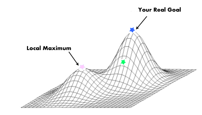
Q: What to do?
- A: Add in some jiggle.
But do not go crazy. As the run goes on, jiggle less and less (so start off jiggling and, over time, become more greedy).
Enter simulated annealling. In the 1950s, when computer RAM was very small, this was a a standard technique for solving non-linear problems. SA generates new solutions by randomly perturbing (a.k.a. “mutating”) some part of an old solution. New replaces old if
- It scores higher;
- or (b) It reaches some probability set by a “temperature” constant.
Initially,this temperature is high so SA jumps to sub-optimal solutions (this allows the algorithm to escape from locally bad ideas).
Subsequently, the “temperature” cools and SA only ever moves to better new solutions.
From Henderson et al. :
- Simulated annealing is so named because of its analogy to the process of physical annealing with solids, in which a crystalline solid is heated and then allowed to cool very slowly until it achieves its most regular possible crystal lattice configuration (i.e., its minimum lattice energy state), and thus is free of crystal defects.
- If the cooling schedule is sufficiently slow, the final configuration results in a solid with such superior structural integrity.
- Simulated annealing establishes the connection between this type of thermo- dynamic behavior and the search for global minima for a discrete optimization problem.
- Furthermore, it provides an algorithmic means for exploiting such a connection.
SA is often used in SBSE, perhaps due to its simplicity. Here's the whole code:
- Let k be some temperature constant that is varied 1 to kmax + So k / kmax is some number 0..1 representing the extent of the current search.
- Let s be a solution (a list of numbers) with energy e.
- Let sn be the next solution with energy en.
- Let sb, se be best solution and energy yet found.
- Let emax be "enough" energy. Usually, max possible minus some epsilon vale.
Code:
s := s0; e := E(s)                  // Initial state, energy.
sb := s; eb := e                    // Initial "best" solution
k := 0                              // Energy evaluation count.
WHILE k < kmax and e > emax         // While time remains & not good enough:
  sn := neighbor(s)                 //   Pick some neighbor.
  en := E(sn)                       //   Compute its energy.
  IF    en < eb                     //   Is this a new best?
  THEN  sb := sn; eb := en          //     Yes, save it.
        print "!"
  FI
  IF    en < e                      // Should we jump to better?
  THEN  s := sn; e := en            //    Yes!
        print "+"
  FI
  ELSE IF P(e, en, k/kmax) < rand() // Should we jump to worse?
  THEN  s := sn; e := en            //    Yes, change state.
        print "?"
  FI
  print "."
  k := k + 1                        //   One more evaluation done
  if k % 50 == 0: print "\n",sb
RETURN sb                           // Return the best solution found.
Note the space requirements for SA: only enough RAM to hold 3 solutions. Very good for old fashioned machines.
Note the print statements shown above:
- One new line ever 50 steps;
- At the start of each new line, print current best energy
- Print "!" if we get to somewhere better globally;
- Print "+" if we get to somewhere better locally;
- Print "?" if we are jumping to something sub-optimal;
So, for a model with one input x and two output goals f1,f2, the run looks like this. Note that each line is a report after k=50 new steps into the simulated annealling.
51 ..!+.?.+..?.+..!+.?.+.?.!+..?.+.?..?..?...+.?.?.+.+...?.+..+.......?...+....+..
99 ....+.+.....?.+..+....?...!+..........?.+......+..........?..+.+
99 .....?..+...+..+......+......+..........?.+...+.........!+...
99 ...!+..?.+..........+.......?....+...+.......+......?.+......
99 ........?......+.......+.....?.+.+.........?.+...+..+.......
99 ........?....+.....+.?..+.+..?...+.........+...+............
99 ....+.......?....+..+....?.+.....+......?.+..+....+..+........
99 .........+..............?.+..+........................
99 ....+.......................?..+.+.+.....+..............
99 ...?.+.+...........!+...............?.+.+..........+.......
99 ......+..................+..................+......+..
99 ....................?...+.+..+........................
99 ........?.+..+.............+.................?..+.......
99 ...+...............................................
99 ...............................................?.+..
99 .+................+.................................
99 .!+.................................................
99 ...........................?.?.+......+...............
99 ..................................................
99 ..................................................
Note that there are less "?" marks (crazy jumps) later in the run than earlier. This is the result of the cooling schedule adjusting the temperature.
Note also that it looks like we are wasting our time after the first 50 evaluations. But as shown below, that is the fault of the summary variable we are using for energy. It turns out that important things are happening even into the 8th and 12th line (500 to 600 evaluations).
Over that run, out two goals changed as follows. As before, each line is a report after k=50 new steps into the simulated annealling. Note how, initially, the median values and variances are very very large. But after a few lines, we get down to very low values and very low variances.
(Btw, to read the following, "*" is the median 50% value; the upper and lower quintiles are shown as "-" left and right; and the other quintiles are shown as white space.)
<f1
                            10%  30%   50%   70%   90%
						    ==========================
   *      --|---------   ,  32,  159, 1558, 4128, 9052
 * ---------|---         ,   5,  100,  515, 1332, 6622
 * ---------|----        ,   3,  239,  467, 1255, 7075
*-          |            ,   2,    2,    2,  167,  874
*--         |            ,  18,   18,   18,  647, 1569
 *          |            ,  18,   48,  427,  427,  586
  *--       |            ,  65,  170, 1087, 1087, 2168
*           |            ,  18,   50,   50,   50,   50
*           |            ,   8,   18,   18,   18,   18
*           |            ,   8,    8,   53,   53,  302
*           |            ,  16,   16,   16,   40,   53
*           |            ,   6,    6,    6,   65,   65
*           |            ,   0,   65,   65,   65,  114
*           |            ,   0,    0,    0,    0,    0
 *          |            ,   0,   35,  635,  635,  791
*           |            ,  20,   33,   73,  405,  592
*           |            ,   1,    1,    1,    1,  351
*           |            ,   1,  126,  126,  126,  501
*           |            ,   8,    8,    8,    8,    8
*           |            ,   0,    0,    1,    8,    8
<f2
                            10%  30%   50%   70%   90%
						    ==========================
    *     --|---------   ,  14,  214, 1720, 4389, 9437
 * ---------|---         ,   0,   64,  610, 1482, 6952
 *----------|---         ,  14,  181,  558, 1118, 6743
*-          |            ,   1,    1,    1,  222,  996
*--         |            ,   5,    5,    5,  753, 1415
*           |            ,   5,   80,  349,  349,  493
  *--       |            ,  37,  226,  959,  959, 2359
*           |            ,  25,   25,   25,   39,   39
*           |            ,   1,   39,   39,   39,   39
*           |            ,   1,    1,   28,   28,  237
*           |            ,  19,   28,   36,   36,   36
*           |            ,  20,   20,   20,  102,  102
*           |            ,   4,  102,  102,  102,  161
*           |            ,   4,    4,    4,    4,    4
 *          |            ,   4,   63,  538,  538,  683
*           |            ,   6,   14,   43,  490,  593
*           |            ,   1,    1,    1,    1,  430
*           |            ,   1,   85,   85,   95,  415
*           |            ,   1,    1,    1,    1,    1
*           |            ,   1,    1,    1,    3,    3
So one lesson from the above- it is not be enough to judge an optimizer just by the average performance. Note in the above that the variance is also an important factor, as is the upper bound (worst case performance) that may take some time to tame.
But what to us for the probability function "P"? This is standard function:
FUNCTION P(old,new,t) = e^((old-new)/t)
Which, incidentally, looks like this (note that the volume where we might jump to a worse solution shrinks as the temperature increases:
Initially at k=0, (t=0):

Subsequently k=0.5*kmax (t=0.5):

Finally at k=kmax (t=1):

That is, we jump to a worse solution when "random() > P" in two cases:
- The sensible case: if "new" is greater than "old"
- The crazy case: earlier in the run (when "t" is small)
Note that such crazy jumps let us escape local minima.