These notes will show an overview of the process by which you can prepare your data for further analysis, as well as how you can further get to know your data. Some steps of this process are not fun at all, but they are an important part of the data science pipeline.
Data Cleaning: the process by which you "tame" your "wild" data. This is an important step of the process because it is at this step where measurement is determined. (e.g. "how many cigarettes per day do I define to be 'smoking'?")
You may do the following steps during the data cleaning process:
- Convert file format
- e.g. JSON to CSV
- Rectangularize your data
- e.g. store in data frame (or other useful container)
- Clean up string variables
- e.g. remove "stop words" like "the," remove punctuation, keep only word stems
- Convert format of variables for downstream use
- e.g. convert dates to specific format
- Normalize values of numerical data
- e.g. standard deviation units
- Impute missing values
- Merge with other existing data sources
- Remove outlier observations
- e.g. by top- or bottom-coding aka winsorizing
- Fix typos in numeric variables
- e.g.
5.25instead of525
- e.g.
- Browse the data
Data Exploration: the process by which you more fully inspect your data. Data cleaning and data exploration constitute an interative process. (Yet another reason to make sure you write code that is reproducible!)
Data exploration includes the following steps:
- Computing descriptive statistics
- e.g. mean, variance, min, max, median, etc.
- Creating frequency tables
- e.g. to tell if a variable is continuous or discrete
- Creating transformations of existing variables
- e.g.
x^2,ln(x), etc.
- e.g.
- Creating new variables from combinations of existing variables
- e.g.
x*z,x*w*z, etc. - This is also called "feature engineering"
- e.g.
- Visualizing your data
- e.g. charts, graphs, scatter plots, etc.
- Running preliminary models
- e.g. pairwise correlations, regressions, etc.
- Selecting subsamples
- e.g. throw out baby boomers because millenials are the population of interest
Throughout the process of data cleaning/exploration, you should constantly be asking yourself the following questions:
- What is my unit of analysis?
- How am I measuring the phenomena I am attempting to research?
- Do the variables mean what I think they should mean?
- Does my data set have the expected number of observations?
- What fraction of values are missing in my data? Is this what I would have expected?
- Are variables named in such a way that if I were to give this data set to someone else, they would understand the contents of the data?
- Are the variables I am interested in continuous or discrete?
- Does anything about my data look funny?
Often, it will be useful to normalize your data in specific ways. Why is it advantaeous to normalize numerical data?
- It often greatly enhances numerical performance
- It can help you interpret your model's results down the line (i.e. "A one-unit increase in X corresponds to a one-standard-deviation increase in Y")
This is done by computing z = (x-mu)/sigma where mu is the sample average and sigma is the sample standard deviation. The resulting variable takes on values typically between -5 and +5, and each unit is interpreted as one standard deviation.
example In education data, student test scores are often expressed in z-score units to facilitate "apples to apples" comparisons
In data science applications, many ML algorithms require z-scored data to appropriately run. This is because unscaled data can sometimes cause numerical issues. Some ML packages will do this z-scoring for the user as part of the algorithm.
This is done by normalizing the variable relative to its max and min. The transformed variable takes on values in [0,1]:
z = (x-min(x))/(max(x)-min(x))
The issue with this method is that if your data set has crazy outliers, 95% of the data will be clustered at 0.5 in the normalized variable.
This is another way to transform a variable to fall in the (0,1) interval. This method is immune to outliers:
z = exp(x)/(1+exp(x))
or equivalently
z = 1/(1+exp(-x))
It's called sigmoidal because the function f(x) = 1/(1+exp(-x)) is known as the sigmoid (or logistic) function.
If one wanted to normalize a variable to fall in the interval (-k,k), one can use the hyperbolic tangent function:
z = k*tanh(x)
This is a lot like the sigmoid function, only it goes from (-k,k) instead of (0,1).
Sometimes, it's useful to convert a continuous variable into a discrete one. This can be done in a myriad of ways. (We won't cover these in detail, but think of how a histogram is built.)
It may also help to transform variables to fit your specific needs. One common transformation is the log transformation:
z = ln(x)
If you are examining earnings, sales, or some other nominal currency quantity, these distributions often are approximately log-normal. If you take the log of a log-normal distribution, you get back a normal distribution, which is very convenient to work with.
In general, you should think "log-normal" if you see a variable that is:
- continuous
- always positive
- has a lot of observations clustered around a small(ish) value
- has a really, really long tail
So you've got some missing values in your data. What can you do to fix them?
- Listwise deletion
- Mean (or mode) substitution
- Regression (or k-nearest neighbors) matching
- Multiple imputation
- Bayesian methods
- Create a binary variable indicating missingness and use it as a control in downstream models
- Interpolate missing values (very useful for panel data!)
The key to choosing an imputation scheme is knowing why the values are missing in the first place. Are they missing e.g. because users randomly had a glitch that kicked them off the website? Or are they missing because some users didn't feel like clicking "purchase" and instead logged off, leaving the product in their cart?
There are three types of "missingness":
- Missing Completely At Random (MCAR): values are missing for completely random reasons. i.e. a weighted coin was flipped which determined whether the value made it into our data set
- Think of this like a randomized experiment
- Missing At Random (MAR): values are not missing at random, but we can account for their missingness by using variables for which we have information
- like a regression model which satisfies the unconfoundedness assumption
- Missing Not At Random (MNAR): values are missing for reasons that are not random, and which cannot fully be accounted for by other variables for which we have information
- like an endogenous choice which is made based on utility maximization
- sample selection bias
- canonical example: only observe wages for people who are employed; employment is not randomly assigned
- newer example: only observe tweets of twitter users; twitter accounts (and usage) not randomly assigned
If the values are missing completely at random (MCAR) then we can simply drop the entire offending row and our final results will not be biased.
The downside is that we will lose statistical power (because we will have fewer observations)
Also, if lots of variables are MCAR in different ways, this can drastically reduce the number of observations.
Another way to impute missing values is to fill in missings with the mean (if variable is continuous) or the mode (if variable is discrete).
This is not a great way to fix the problem. On the one hand, the average (mode) is unchanged. On the other hand, the variance is severely deflated.
One can also impute by picking another observation for which the value is not missing, and which all other variables are as similar as possible.
Essentially, we find a "donor" for the observation that is missing, and say "If the observations look similar enough, we can plug in the donor's non-missing value."
We can use a number of ways to find the donor: OLS, k-nearest neighbors, random forest, etc.
This method works great if values are MAR.
It is important to keep in mind that these model-based imputation methods may understate the true variance of the distribution, so it is sometimes helpful to inject noise into the imputed values.
Multiple imputation is a multi-step process:
- Impute values M different times (via any of the above methods)
- With M different data sets, conduct your analysis on each data set
- Consolidate analyses (e.g. by averaging)
Example: MICE (Mulitple Imputation by Chained Equations)
At the end of the day, most multiple imputation methods are variations on "matching" which requires MAR.
Another way to impute is to use Bayesian methods. The R package MixedDataImpute uses a state-of-the-art statistical model to impute missing values. Its performance exceeds that of MICE and other multiple imputation methods.
My preferred way to impute is to create a new variable that is 1 when the values of x are missing, and 0 otherwise.To create this, I follow these two steps:
- Create the variable (e.g.
m_x) equal to 1 ifxis missing, 0 otherwise. - Recode the missing values of
xto be some constant value outside the support (e.g. 50)
The key thing to remeber is that x now has a mass point at 50, so when computing summary statistics, you should exclude these observations.
The nice thing about this is that you can, for example, run a regression and include m_x as a control variable, and it will estimate a separate effect for x for the group of values that are missing.
If one has repeated observations of the same unit, one can fill in the values by interpolating.
Example from my research:
- follow individuals over extended period of time
- in some years (e.g. 2010), individuals don't report their earnings
- but I can see that they are working at the same job in 2009 and 2011, and I see their earnings in those years
- I can interpolate their 2010 earnings by taking the average of the 2009 and 2011 earnings
Note: Interpolation requires having valid values on each boundary point. If you don't have this, then it's called extrapolation and it's much more prone to error.
In my example above, if I observed earnings in 2009 and 2010, but not 2011, I would not be comfortable setting 2011 earnings to be the average of 2009 and 2010 because the individual may have gotten a promotion, etc.
Descriptive statistics (mean, median, variance, min, max) may seem "boring" but they are the easiest way for you to summarize your data.
It's often helpful to generate a summary table that lists the descriptive statistics for each of the variables you are studying (either outcomes or controls). For example:
| Variable | Obs. | Mean | Std. Dev. | Median | Min | Max |
|---|---|---|---|---|---|---|
| Sales | 15,147 | 13,456.50 | 16,579.81 | 10,500.00 | 501.00 | 165,789.00 |
| Morning | 363,528 | 0.24 | 0.43 | 0.00 | 0.00 | 1.00 |
| Afternoon | 363,528 | 0.36 | 0.48 | 0.00 | 0.00 | 1.00 |
| Evening | 363,528 | 0.35 | 0.48 | 0.00 | 0.00 | 1.00 |
| Night | 363,528 | 0.05 | 0.22 | 0.00 | 0.00 | 1.00 |
| Income | 363,528 | 96,501.73 | 87,389.19 | 82,000.00 | 23,000.00 | 425,000.00 |
| Age | 363,528 | 55.87 | 12.77 | 52.00 | 14.00 | 96.00 |
| Female | 363,528 | 0.42 | 0.49 | 0.00 | 0.00 | 1.00 |
Anything wrong with this table? Anything that jumps out at you?
It's often helpful to compute frequency tables of each of your variables that are discrete (categorical).
This will help you visualize the distribution of these variables. For example:
- Is the distribution of this three-category variable roughly uniform?
- Or are 95% of the values in one of the three categories?
It often helps to run preliminary statistical models to see how your variables covary, how sensitive raw correlations are to inclusion of additional predictors, etc.
- pairwise correlations (including rank correlations)
- concordance indices (e.g. Jaccard similarity)
- OLS
- Logit, Probit, etc.
We'll talk more about these next week
Commonly used data visualization types that are useful in getting to know your data:
- box-and-whisker plot
- scatter plot
- histogram
- kernel density plot
- binned scatter plots (aka "binscatter")
- line charts
- maps
- summary tables (tables are a visualization tool!)
- word clouds (for textual data)
- many others
Different visualization tools can be used for different tasks:
- Find outliers
- Examine distribution of values
- box-and-whisker, histogram, kernel density
- Report correlations
- scatter plot or binscatter (for two continuous variables)
- plots by "facet" (for one continuous variable and one categorical variable)
- Examine trends in time series data
- line charts
- Text trends
- word clouds
- word trees
See here for a step-by-step guide on the basics of creating data visuals in R using ggplot2.
R package for binscatters: binscattr (still in its infancy)
This website has a nice summary of types of visuals that may be helpful in telling your story.


More beautiful visualizations available at r/dataisbeautiful
Comical opponent: r/dataisugly
- You don't want to end up on that site
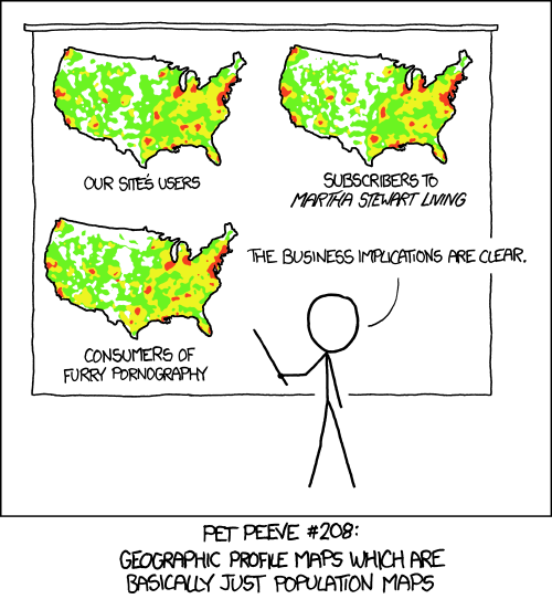
Always make sure that your image conveys useful information
This module of the course covers data visualization tools. We'll learn these tools by studying economic mobility using data from the Equality of Opportunity Project.
Where is the Land of Opportunity? The Geography of Intergenerational Mobility in the United States