In order to set up the workflow and generate an experiment with the SRW Application, the user must choose between various predefined FV3-LAM grids or generate a user-defined grid. At this time, full support is only provided to those using one of the five predefined grids supported in the release, but other predefined grids are available (see Section %s <PredefGrid> for more detail). Preliminary information is also provided at the end of this chapter describing how users can leverage the SRW App workflow scripts to generate their own user-defined grid and/or to adjust the number of vertical levels in the grid. Currently, these features are not fully supported and are "use at your own risk."
The SRW App includes five predefined limited area model (LAM) grids. To select a supported predefined grid, the PREDEF_GRID_NAME variable within the workflow: section of the config.yaml script must be set to one of the following five options:
RRFS_CONUS_3kmRRFS_CONUS_13kmRRFS_CONUS_25kmSUBCONUS_Ind_3kmRRFS_NA_13km
These five options are provided for flexibility related to compute resources and supported physics options. Other predefined grids are listed here <PredefGrid>. The high-resolution 3-km CONUS grid generally requires more compute power and works well with three of the five supported physics suites (see Table %s <GridPhysicsCombos>). Low-resolution grids (i.e., 13-km and 25-km domains) require less compute power and should generally be used with the other supported physics suites: FV3_GFS_v16 and FV3_RAP.
| Grid | Physics Suite(s) |
|---|---|
| RRFS_CONUS_3km | FV3_RRFS_v1beta FV3_HRRR FV3_WoFS |
| SUBCONUS_Ind_3km | FV3_RRFS_v1beta FV3_HRRR FV3_WoFS |
| RRFS_CONUS_13km | FV3_GFS_v16 FV3_RAP |
| RRFS_NA_13km | FV3_RAP FV3_GFS_v16 |
| RRFS_CONUS_25km | FV3_GFS_v16 FV3_RAP |
In theory, it is possible to run any of the supported physics suites with any of the predefined grids, but the results will be more accurate and meaningful with appropriate grid/physics pairings.
The predefined CONUS grids follow the naming convention (e.g., RRFS_CONUS_*km) of the 3-km version of the continental United States (CONUS) grid being tested for the Rapid Refresh Forecast System (RRFS). RRFS will be a convection-allowing, hourly-cycled, FV3-LAM-based ensemble planned for operational implementation in 2025. Aside from RRFS_NA_13km, the supported predefined grids were created to fit completely within the High Resolution Rapid Refresh (HRRR) domain to allow for use of HRRR data to initialize the SRW App. The RRFS_NA_13km grid covers all of North America and therefore requires different data to initialize.
The 3-km CONUS domain is ideal for running the FV3_RRFS_v1beta physics suite, since this suite definition file (SDF) was specifically created for convection-allowing scales and is the precursor to the operational physics suite that will be used in RRFS. The 3-km domain can also be used with the FV3_HRRR and FV3_WoFS physics suites, which likewise do not include convective parameterizations. In fact, the FV3_WoFS physics suite is configured to run at 3-km or less and could therefore run with even higher-resolution user-defined domains if desired. However, the FV3_GFS_v16 and FV3_RAP suites generally should not be used with the 3-km domain because the cumulus physics used in those physics suites is not configured to run at the 3-km resolution.
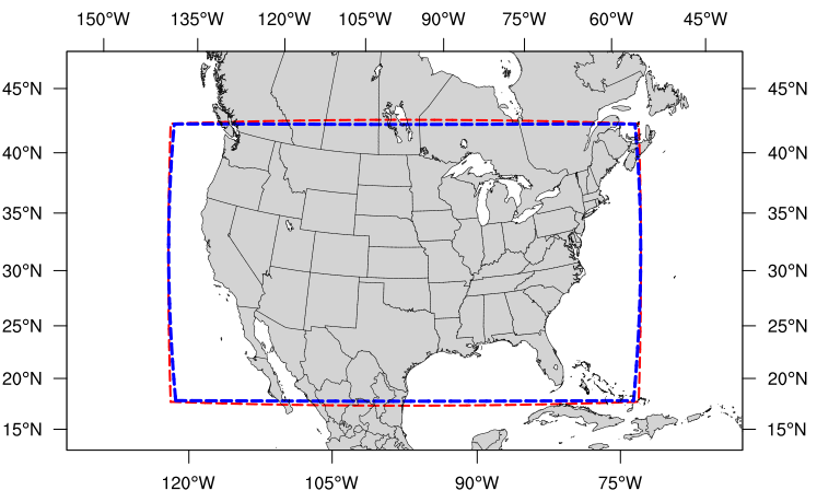 The boundary of the RRFS_CONUS_3km computational grid (red) and corresponding write component grid (blue).
The boundary of the RRFS_CONUS_3km domain is shown in Figure %s <RRFS_CONUS_3km> (in red), and the boundary of the write component grid <WriteComp> sits just inside the computational domain (in blue). This extra grid is required because the post-processing utility (UPP) is unable to process data on the native FV3 gnomonic grid (in red). Therefore, model data are interpolated to a Lambert conformal grid (the write component grid) in order for the UPP to read in and correctly process the data.
Note
While it is possible to initialize the FV3-LAM with coarser external model data when using the RRFS_CONUS_3km domain, it is generally advised to use external model data (such as HRRR or RAP data) that has a resolution similar to that of the native FV3-LAM (predefined) grid.
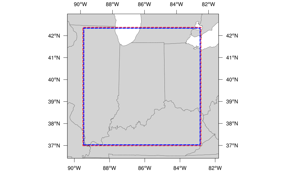 The boundary of the SUBCONUS_Ind_3km computational grid (red) and corresponding write component grid (blue).
The SUBCONUS_Ind_3km grid covers only a small section of the CONUS centered over Indianapolis. Like the RRFS_CONUS_3km grid, it is ideally paired with the FV3_RRFS_v1beta, FV3_HRRR, or FV3_WoFS physics suites, since these are all convection-allowing physics suites designed to work well on high-resolution grids.
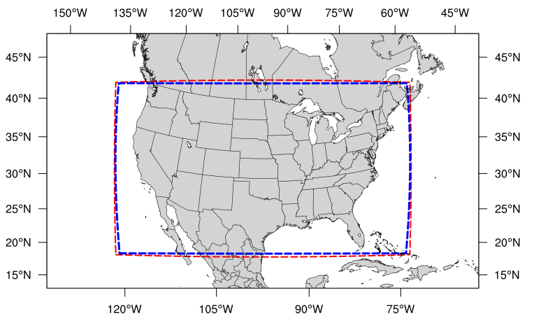 The boundary of the RRFS_CONUS_13km computational grid (red) and corresponding write component grid (blue).
The RRFS_CONUS_13km grid (Fig. %s <RRFS_CONUS_13km>) covers the full CONUS. This grid is meant to be run with the FV3_GFS_v16 or FV3_RAP physics suites. These suites use convective parameterizations, whereas the other supported suites do not. Convective parameterizations are necessary for low-resolution grids because convection occurs on scales smaller than 25-km and 13-km.
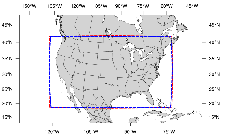 The boundary of the RRFS_CONUS_25km computational grid (red) and corresponding write component grid (blue).
The RRFS_NA_13km grid (Fig. %s <RRFS_NA_13km>) covers all of North America. This grid was designed to run with the FV3_RAP physics suite but can also be run with the FV3_GFS_v16 suite. These suites use convective parameterizations, whereas the other supported suites do not. Convective parameterizations are necessary for low-resolution grids because convection occurs on scales smaller than 25-km and 13-km.
Corner plots for the RRFS_NA_13km grid in Table %s <CornerPlots> show the 4-cell-wide halo on the computational grid in orange, which gives an idea of the size of the grid cells.
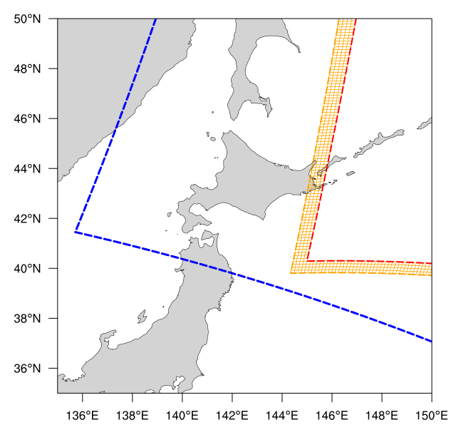
Upper left w/halo
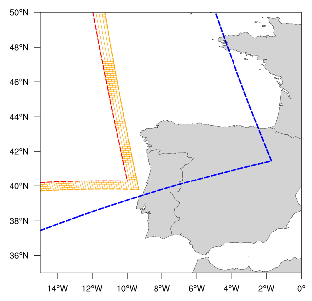
Upper right w/halo
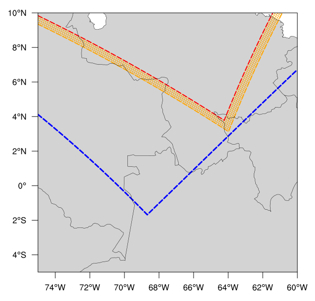
Lower right w/halo
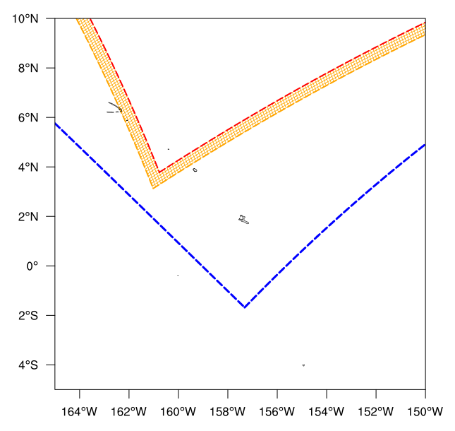
Lower left w/halo
The boundary of the RRFS_CONUS_25km computational grid (red) and corresponding write component grid (blue).
The final predefined CONUS grid (Fig. %s <RRFS_CONUS_25km>) uses a 25-km resolution and is meant mostly for quick testing to ensure functionality prior to using a higher-resolution domain. However, if users plan to use the 25-km domain for research, the FV3_GFS_v16 SDF is recommended for the reasons mentioned above <RRFS_CONUS_13km>.
Ultimately, the choice of grid is experiment-dependent and resource-dependent. For example, a user may wish to use the FV3_GFS_v16 physics suite, which uses cumulus physics that are not configured to run at the 3-km resolution. In this case, the 13-km or 25-km domain options are better suited to the experiment. Users will also have fewer computational constraints when running with the 13-km and 25-km CONUS domains, so depending on the resources available, certain grids may be better options than others.
While the five supported predefined grids are ideal for users just starting out with the SRW App, more advanced users may wish to create their own predefined grid for testing over a different region and/or with a different resolution. Creating a user-defined grid requires knowledge of how the SRW App workflow functions. In particular, it is important to understand the set of scripts that handle the workflow and experiment generation (see Figure %s <WorkflowGeneration> and Figure %s <WorkflowTasksFig>). It is also important to note that user-defined grids are not a supported feature of the current release; however, information is being provided for the benefit of the FV3-LAM community.
With those caveats in mind, this section provides instructions for adding a new predefined grid to the FV3-LAM workflow that will be generated using the "ESGgrid" method (i.e., using the regional_esg_grid code in the UFS_UTILS repository, where ESG stands for "Extended Schmidt Gnomonic"). We assume here that the grid to be generated covers a domain that (1) does not contain either of the poles and (2) does not cross the -180 deg --> +180 deg discontinuity in longitude near the international date line. More information on the ESG grid is available here <Purser_UIFCW_2023.pdf>. Instructions for domains that do not have these restrictions will be provided in a future release.
The steps to add such a grid to the workflow are as follows:
- Choose the name of the grid. For the purposes of this documentation, the grid will be called "NEW_GRID".
- Add NEW_GRID to the array
valid_vals_PREDEF_GRID_NAMEin theufs-srweather-app/ush/valid_param_vals.yamlfile. - In
ufs-srweather-app/ush/predef_grid_params.yaml, add a stanza describing the parameters for NEW_GRID. An example of such a stanza is givenbelow <NewGridExample>. For descriptions of the variables that need to be set, see Sections%s: ESGgrid Settings <ESGgrid>and%s: Forecast Configuration Parameters <FcstConfigParams>.
To run a forecast experiment on NEW_GRID, start with a workflow configuration file for a successful experiment (e.g., config.community.yaml, located in the ufs-srweather-app/ush subdirectory), and change the line for PREDEF_GRID_NAME in the workflow: section to NEW_GRID:
PREDEF_GRID_NAME: "NEW_GRID"Then, load the workflow environment, specify the other experiment parameters in config.community.yaml, and generate a new experiment/workflow using the generate_FV3LAM_wflow.py script (see Section %s <GenerateForecast> for details).
The following is an example of a code stanza for "NEW_GRID" to be added to predef_grid_params.yaml:
#
#---------------------------------------------------------------------
#
#  Stanza for NEW_GRID. This grid covers [description of the
#  domain] with ~[size]-km cells.
#
#---------------------------------------------------------------------

"NEW_GRID":

# The method used to generate the grid. This example is specifically for the "ESGgrid" method.


  GRID_GEN_METHOD: "ESGgrid"

# ESGgrid parameters

  ESGgrid_LON_CTR: -97.5
  ESGgrid_LAT_CTR: 38.5
  ESGgrid_DELX: 25000.0
  ESGgrid_DELY: 25000.0
  ESGgrid_NX: 200
  ESGgrid_NY: 112
  ESGgrid_PAZI: 0.0
  ESGgrid_WIDE_HALO_WIDTH: 6

# Forecast configuration parameters

  DT_ATMOS: 40
  LAYOUT_X: 5
  LAYOUT_Y: 2
  BLOCKSIZE: 40

# Parameters for the write component (aka "quilting") grid.

  QUILTING:
    WRTCMP_write_groups: 1
    WRTCMP_write_tasks_per_group: 2
    WRTCMP_output_grid: "lambert_conformal"
    WRTCMP_cen_lon: -97.5
    WRTCMP_cen_lat: 38.5
    WRTCMP_lon_lwr_left: -121.12455072
    WRTCMP_lat_lwr_left: 23.89394570

# Parameters required for the Lambert conformal grid mapping.

    WRTCMP_stdlat1: 38.5
    WRTCMP_stdlat2: 38.5
    WRTCMP_nx: 197
    WRTCMP_ny: 107
    WRTCMP_dx: 25000.0
    WRTCMP_dy: 25000.0
Note
The process above explains how to create a new predefined grid, which can be used more than once. If a user prefers to create a custom grid for one-time use, the variables above can instead be specified in config.yaml, and PREDEF_GRID_NAME can be set to a null string. In this case, it is not necessary to modify valid_param_vals.yaml or predef_grid_params.yaml. Users can view an example configuration file for a custom grid here.
The five supported predefined grids included with the SRW App are configured to run with 65 levels by default. However, advanced users may wish to vary the number of vertical levels in the grids they are using, whether these be the predefined grids or a user-generated grid. Varying the number of vertical levels requires knowledge of how the SRW App interfaces with the UFS Weather Model (WM <Weather Model>) and preprocessing utilities. It is also important to note that user-defined vertical levels are not a supported feature at present; information is being provided for the benefit of the FV3-LAM community, but user support for this feature is limited. With those caveats in mind, this section provides instructions for creating a user-defined vertical coordinate distribution on a regional grid.
Users will need to determine ak and bk values, which are used to define the vertical levels. The UFS WM uses a hybrid vertical coordinate system, which moves from purely sigma levels near the surface to purely isobaric levels near the top of the atmosphere (TOA). The equation pk = ak + bk * ps (where ps is surface pressure) is used to derive the pressure value at a given level. The ak values define the contribution from the purely isobaric component of the hybrid vertical coordinate, and the bk values are the contribution from the sigma component. When ak and bk are both zero, it is the TOA (pressure is zero). When bk is 1 and ak is 0, it is a purely sigma vertical coordinate surface, which is the case near the surface (the first model level).
The vcoord_gen tool from UFS_UTILS can be used to generate ak and bk values, although users may choose a different tool if they prefer. The program can output a text file containing ak and bk values for each model level, which will be used by chgres_cube in the make_ics_* and make_lbcs_* tasks to generate the initial and lateral boundary conditions from the external data.
Users can find vcoord_gen technical documentation here and scientific documentation here. Since UFS_UTILS is part of the SRW App, users can find and run the UFS_UTILS vcoord_gen tool in their ufs-srweather-app/exec directory. To run vcoord_gen within the SRW App:
cd /path/to/ufs-srweather-app/exec
./vcoord_gen > /path/to/vcoord_gen_outfile.txt
Users should modify the output file path (/path/to/vcoord_gen_outfile.txt) to save the output file in the desired location. In the SRW App, the default file defining vertical levels is named global_hyblev.txt and contains the default 65 levels. By convention, users who create a new vertical coodinate distribution file often append this file name with LXX or LXXX for their number of levels (e.g., global_hyblev.L128.txt). Configuration files are typically placed in the parm directory. For example, a user (Jane Smith) might run:
cd /Users/Jane.Smith/ufs-srweather-app/exec
./vcoord_gen > /Users/Jane.Smith/ufs-srweather-app/parm/global_hyblev.L128.txt
When vcoord_gen starts, it will print a message telling users to specify certain variables for ak/bk generation:
Enter levs,lupp,pbot,psig,ppre,pupp,ptop,dpbot,dpsig,dppre,dpupp,dptopFor an experiment using 128 vertical levels, users might then input:
128,88,100000.0,99500.0,7000.0,7000.0,0.0,240.0,1200.0,18000.0,550.0,1.0After hitting Enter, the program will print a pmin value (e.g., pmin= 50392.6447810470) and save the output file in the designated location. Based on the default values used above, the contents of the file should look like this:
2 1280.000 1.00000000 0.000 0.99752822 0.000 0.99490765 0.029 0.99212990 0.232 0.98918511 0.810 0.98606254 1.994 0.98275079 4.190 0.97923643 8.287 0.97550087
15.302 0.97152399 26.274 0.96728509 42.274 0.96276297 64.392 0.95793599 93.740 0.95278208
131.447 0.94727885 178.651 0.94140368 236.502 0.93513378 306.149 0.92844637 388.734 0.92131872 485.392 0.91372837 597.235 0.90565322 725.348 0.89707176 870.778 0.88796321
1034.524 0.87830771 1217.528 0.86808662 1420.661 0.85728262 1644.712 0.84588007 1890.375 0.83386518 2158.238 0.82122630 2448.768 0.80795416 2762.297 0.79404217 3099.010 0.77948666 3458.933 0.76428711 3841.918 0.74844646 4247.633 0.73197127 4675.554 0.71487200 5124.949 0.69716312 5594.876 0.67886334 6084.176 0.65999567 6591.468 0.64058751 7115.147 0.62067071 7653.387 0.60028151 8204.142 0.57946049 8765.155 0.55825245 9333.967 0.53670620 9907.927 0.51487434
10484.208 0.49281295 11059.827 0.47058127 11631.659 0.44824125 12196.468 0.42585715 12750.924 0.40349506 13291.629 0.38122237 13815.150 0.35910723 14318.040 0.33721804 14796.868 0.31562289 15248.247 0.29438898 15668.860 0.27358215 16055.485 0.25326633 16405.020 0.23350307 16714.504 0.21435112 16981.137 0.19586605 17202.299 0.17809988 17375.561 0.16110080 17498.697 0.14491294 17569.698 0.12957622 17586.772 0.11512618 17548.349 0.10159397 17453.084 0.08900629 17299.851 0.07738548 17088.325 0.06674372 16820.937 0.05706358 16501.018 0.04831661 16132.090 0.04047056 15717.859 0.03348954 15262.202 0.02733428 14769.153 0.02196239 14242.890 0.01732857 13687.727 0.01338492 13108.091 0.01008120 12508.519 0.00736504 11893.639 0.00518228 11268.157 0.00347713 10636.851 0.00219248 10004.553 0.00127009 9376.141 0.00065078 8756.529 0.00027469 8150.661 0.00008141 7563.494 0.00001018 7000.000 0.00000000 6463.864 0.00000000 5953.848 0.00000000 5468.017 0.00000000 5004.995 0.00000000 4563.881 0.00000000 4144.164 0.00000000 3745.646 0.00000000 3368.363 0.00000000 3012.510 0.00000000 2678.372 0.00000000 2366.252 0.00000000 2076.415 0.00000000 1809.028 0.00000000 1564.119 0.00000000 1341.538 0.00000000 1140.931 0.00000000 961.734 0.00000000 803.164 0.00000000 664.236 0.00000000 543.782 0.00000000 440.481 0.00000000 352.894 0.00000000 279.506 0.00000000 218.767 0.00000000 169.135 0.00000000 129.110 0.00000000 97.269 0.00000000 72.293 0.00000000 52.984 0.00000000 38.276 0.00000000 27.243 0.00000000 19.096 0.00000000 13.177 0.00000000 8.947 0.00000000 5.976 0.00000000 3.924 0.00000000 2.532 0.00000000 1.605 0.00000000 0.999 0.00000000 0.000 0.00000000
To use the new ak/bk file to define vertical levels in an experiment, users will need to modify the input namelist file (input.nml.FV3) and their configuration file (config.yaml).
The FV3 namelist file, input.nml.FV3, is located in ufs-srweather-app/parm. Users will need to update the levp and npz variables in this file. For n vertical levels, users should set levp=n and npz=n-1. For example, a user who wants 128 vertical levels would set levp and npz as follows:
&external_ic_nml
   levp = 128

&fv_core_nml
   npz = 127
Additionally, check that external_eta = .true..
Note
Keep in mind that levels and layers are not the same. In UFS code, levp is the number of vertical levels, and npz is the number of vertical levels without TOA. Thus, npz is equivalent to the number of vertical layers. For v vertical layers, set npz=v and levp=v+1. Use the value of levp as the number of vertical levels when generating ak/bk.
To use the text file produced by vcoord_gen in the SRW App, users need to set the VCOORD_FILE variable in their config.yaml file. Normally, this file is named global_hyblev.l65.txt and is located in the fix_am directory on Level 1 systems, but users should adjust the path and name of the file to suit their system. For example, in config.yaml, a user (Jane Smith) might set:
task_make_ics:
   VCOORD_FILE: /Users/Jane.Smith/ufs-srweather-app/parm/global_hyblev.L128.txt
task_make_lbcs:
   VCOORD_FILE: /Users/Jane.Smith/ufs-srweather-app/parm/global_hyblev.L128.txt
Configure other variables as desired and generate the experiment as described in Section %s <GenerateForecast>.