ex03_state_estimation

ex03_state_estimation

Theory Lesson: state estimation

(TODO write it down here)

Sensors for State Estimation

Wheel Odometry

How far did my robot travel based on the number of revolutions my motor did? Calculate it for the simplest case by hand: Only driving forwards. Think about what changes if the robot has a linear and an angular velocity.

What to know about wheel odometry:

• Depends on motion model. Equations are different for Ackermann and differential steering.
• Normally depends on the ground surface, but this is ignored in most software
  1. assumption: The ground is flat
  2. assumption: Wheels have infinite friction. They do not slip over the ground

Task: Find, print and understand the wheel odometry data. What message of which package is used?

IMU

Why is it hard to use linear accelerations for translational changes?

• Integration problems.

Task: Find, print and understand the IMU data. What message of which package is used?

LiDAR

Start Gazebo open RViz and visualize the scan topic in fixed frame base_link. Now drive the robot forward. Can you estimate how far the robot has moved? Hint: The default size of a grid cell in RViz is 1x1 m.

What you have done by intuition is exactly what the task of point cloud registration is trying to solve. Search the internet for "ICP". Small overview:

• Find correspondences between a data set and a model by finding the closest points
• Estimate the transformation parameters by Umeyama or non-linear optimization
• Static environment

Locally registering scans is sometimes referred to as LiDAR odometry. It is a core concept of modern SLAM solutions. We do that later.

Camera

It is also possible to use cameras to completely estimate the state of the robot in 3D. A good overview is given by Wikipedia in the Egomotion estimation GIF:

Fusion

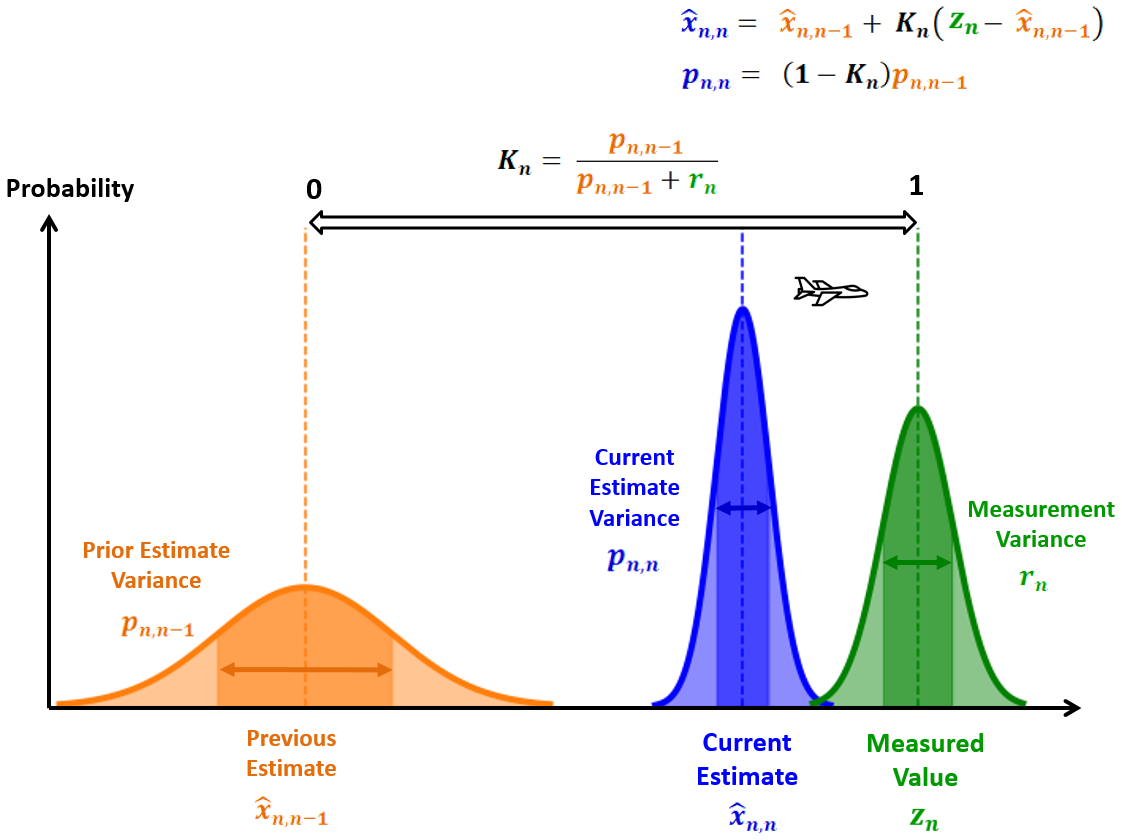
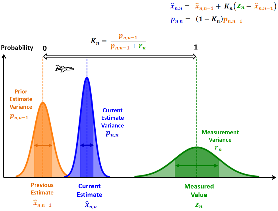
If we have different sensors that all can measure the state of the robot we need to fuse them appropriately. In this case "appropriately" means that we want some measurements to influence parts of our state estimation more than others. For example: We can estimate the translational speed by using the linear acceleration of the IMU or the linear velocity of the wheel odometry. Since we already know linear accelerations are not very reliable when it comes to integrating them to positions, we don't want them to have much influence during fusion. And do not forget: All measurements are noisy. For this, the so-called "Kalman Filter" was invented. It is a simple filter that is a special case of a Bayes-Filter.

This page gives a good overview of how a linear Kalman-Filter works in 1D: https://www.kalmanfilter.net/kalman1d.html :

Linear Kalman-Filters have optimal filtering properties given that

• all the sensors are pefectly modelled
• the system can be modelled by linear transitions
• sensor noise is normal distributed
• the belief state is normal distributed and unimodal

But this is rarely the case in reality. At some point, linear Kalman-Filters are becoming inaccurate because we cannot model the reality well enough. Then one usually switches to Extended Kalman Filters (EKF) or Unscented Kalman Filters (UKF).

On mobile robots, there are most probably running at least one EKF as well. It is oftentimes used to fuse internal sensors, such as IMU and wheel odometry. A Kalman-Filter in general is not something that is the same for every robot. It has to be configured properly to fit the robot's sensors. For example, the ceres robot can be modelled as:

• Use the cmd_vel topic as action / as prior
• Use the odom topic as measurement / as posterior. Linear velocity is less noisy than the rotational velocity
• Use the imu/data_raw as measurement / as posterior. Rotational velocity is far less noisy compared to linear acceleration

Oftentimes the linear acceleration is completely ignored to estimate translational state components. Instead, the linear acceleration is used to improve the angular velocities using e.g. a Madgwick Filter.

With the simulation, we already started a pre-configured EKF from the package robot_localization

The result is the state of the robot given as odometry/filtered topic or as tf-transform odom -> base_footprint.

Task: Open RViz. Switch to fixed frame odom and enable the laser scan. Drive around and see that the robot is localizing well in RViz.

Make yourself familiar with the way the EKF was started and parameterized. New things that you should see:

• Launch files, written in Python
• Parameters defined in YAML files

Task 1: Try to change those parameters a little. For example: Try to enable the linear acceleration of the IMU as an additional measurement

Task 2: Try to integrate such a robot_localization launch and configuration files into this package

Real Robot

Caution !!!: To continue you will be required to press the red emergency stop button at least once.

Now it's time to go to the real robot. You will need at least one laptop, with everything installed, and registered in the same WiFi as the robot (RoboNet).

First try to ping the robot in the network:

ping flamara.informatik.uos.de

Then connect via SSH

ssh robot@flamara.informatik.uos.de

Figure out the ROS_DOMAIN_ID of the robot and set your laptop to the same.

TMUX

Next, you need to learn a tool called tmux. It should be already installed on the robot. You do not necessarily need to install it on your own system. But I recommend installing it anyway in case you want to learn the commands on your own machine first.

sudo apt-get install tmux

Why tmux? Accessing the robot via SSH alone has a few drawbacks:

• If your SSH connection dies so is all you have started
• If you start some nodes, only you can kill or restart them easily

Fortunately, tmux has you covered:

• Start tmux session by calling tmux new -s mysession
  • You will enter the tmux environment: You can recognize it via a green line at the bottom of the terminal
• Leave a session and keep it alive: [CTRL+b] to enter the command mode. Then press [d] (d for detach).
• To enter it again use tmux a (a for attach) and press enter.
• Leave it again and try to create a second session
• Enter it and switch sessions via [CTRL+b] to enter the command mode. Then press [s]. To open a list of available sessions. Select one via the arrow keys and press enter to enter it.

There are more commands but these are the most essential you will need. Such tmux sessions keep alive even after you have lost your SSH connections. Furthermore, its possible to enter one session with more than one user.

Task: One person is creating a tmux session the other person is accessing it. Try to edit a file together.

Bringup

To start everything on the real robot, start a tmux session and call

ros2 launch ceres_bringup ceres_launch.py

This launch file starts all the sensor drivers and an EKF for state estimation. The created topics have the same name and message types as the Gazebo simulation was creating. So all of your already written nodes should work without changing the code.

Task: Test some of your nodes. First, start them on your laptop. Second, transfer the source code to the robot (scp), build it on the robot, and run it on the robot. What is better?

Control the robot via ros2 launch uos_diffdrive_teleop key.launch. One person always(!) has to be ready to push the red button.

RViz with real robot

Start RViz to visualize the real robot's sensor data. Check if the localization via EKF works.

Simulation and Reality

Because of the available ROS2 abstractions, it becomes possible to implement every piece of software just by using the simulation. So home office is possible, isn't it? No. simulated worlds are usually very much simplified and sensor data includes way less noise than reality. Most of the robotics algorithms have to be tested in reality! However, experienced robotics engineers can write software so that it is almost always working in reality.

Preview Mapping

Using either simulated or real robot. Try the following:

Open RViz, set the fixed frame to odom. Visualize a laser scan or a point cloud. Increase the "decay time" to 100. Move around.

Although no active matching of the scans is done, it looks as if the scans match very well. After a time it looks like we are building some kind of a floor plan: a 2D map.

Maps

A map is useful for a robot. It uses it for more robust localization and efficient navigation planning. Maps can exist in various forms. Most of the robots in the world use so-called 2D grid maps, including your vacuum cleaners. More interesting for research, however, are the 3D map formats such as:

• point cloud maps
• voxel maps
• tsdf maps
• mesh maps
• NERFs, NDFs

Try to figure out what is behind those map formats.

For simplicity, we stay in a 2D world. What message is used for a 2D grid map?

SLAM

Simultaneous localization and mapping (SLAM) deal with localizing the robot and at the same time creating a globally consistent map. A quick overview of what has worked out pretty well so far:

1. Using some kind of intrinsic state estimation as prior (Wheel & IMU - EKF)
2. Using scan registration as posterior
3. 1 & 2 tend to drift: Try to detect loops and correct the drift afterward using e.g. pose graph optimization

Assumptions of (most) SLAM:

• Belief state must be unimodal -> first pose has to be known
• What if not? We come back to that later (see MCL)

Ceres robot has implemented a SLAM. Task: Start it by executing:

ros2 launch ceres_localization slam_toolbox_launch.py

Open the tf tree

ros2 run rqt_tf_tree rqt_tf_tree

and explain what has been added. Then run RViz and visualize the map while driving the robot around. Try to save the map.