The R package EpiILM provides tools for simulating from discrete-time individual level models for infectious disease data analysis. This epidemic model class contains spatial and contact-network based models with two disease types: Susceptible-Infectious (SI) and Susceptible-Infectious-Removed (SIR).
You can install the EpiILM version from CRAN.
install.packages('EpiILM', dependencies = TRUE)You can install the development version from Github
# install.packages("devtools")
devtools::install_github("waleeedalmutiry/EpiILM")The key functions of the R package EpiILM is focused on simulating from, and carrying out Bayesian MCMC-based statistical inference for, spatial or, network-based discrete-time individual-level models (ILMs) of infectious disease transmission as proposed by Deardon et al. (2010). The implemented ILMs framework in this package can be set in either susceptible-infected (SI) or susceptible-infected-removed (SIR) compartmental frameworks. For more details about the ILMs, see (Deardon et al., 2010). Table (1) illustrate the key functions of this package in which some of them, including for epidemic simulation and likelihood calculation, are coded in Fortran in order to achieve the goal of agile implementation.
In EpiILM, ILMs can be fitted to observed data within a Bayesian framework. A Metropolis-Hastings MCMC algorithm is used to estimate the posterior distribution of the parameters. This can be done via the epimcmc function which depends on the MCMC function from the adaptMCMC package.
In the following section, we illustrate the use of some of the key features of the EpiILM package in the context of both spatial, and network-based, ILMs.
We start with generating the XY coordinates of 256 individuals coordinates uniformly across a 10 by 10 unit square area. This simulated population is for illustrative purposes, the population data usually being imported for real problems.
library("EpiILM")

set.seed(789)

# generating the XY coordinates of individuals:
x  <-  runif(256,  0, 100)
y  <-  runif(256,  0, 100)
We consider the SI spatial-based ILMs with one susceptibility covariate and no transmissibility covariates to be simulated from. First, let us generate a susceptibility covariate.
A <- round(rexp(256, 1/100))We can then generate the epidemic with two susceptibility parameters (sus.par), and one spatial parameter (beta).
out_cov <- epidata(type = "SI", n = 256, tmax = 10, x = x, y = y,
Sformula = ~A, sus.par = c(0.01, 0.05), beta = 2)
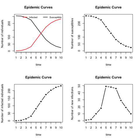
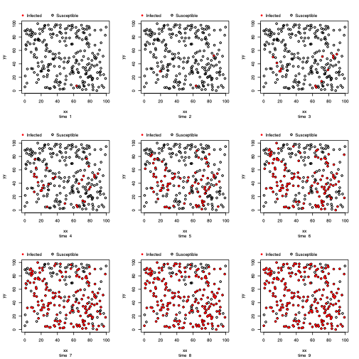
out_covWe introduce an S3 method plot function to illustrate the spread of the epidemic over time. The function can produce various epidemic curves by setting the argument plottype = "curve", and the spatial propagation over time when the model is spatial-based by setting the argument plottype = "spatial". When the plottype = "curve", an additional argument (curvetype) is needed. This is illustrated in the below table.
| curvetype = | Description |
|---|---|
| "complete" | to produce curves of the number of susceptible, infected, and removed (when type = "SIR'') individuals over time. |
| "susceptible" | to produce a single curve for the susceptible individuals over time. |
| "totalinfect" | to produce a cumulative number of infected individuals over time. |
| "newinfect" | to produce a curve of the number of newly infected individuals at each time point. |
par(mfrow=c(2, 2))
plot(out_cov, plottype = "curve", curvetype = "complete")
plot(out_cov, plottype = "curve", curvetype = "susceptible")
plot(out_cov, plottype = "curve", curvetype = "totalinfect")
plot(out_cov, plottype = "curve", curvetype = "newinfect")
plot(out_cov, plottype = "spatial")
Now, we show how to perform an MCMC analysis through the use of the epimcmc function that depends on the MCMC function from the adaptMCMC package.
# to assign the tmax value of the epidemic:
t_end <- max(out_cov$inftime)
# to assign prior distribution for the model parameters:
unif_range <- matrix(c(0, 0, 1, 1), nrow = 2, ncol = 2)
# to perform the MCMC analysis:
mcmcout_M8 <- epimcmc(out_cov, Sformula = ~A,
tmax = t_end, niter = 50000,
sus.par.ini = c(0.03, 0.005), beta.ini = 2,
pro.sus.var = c(0.005, 0.005), pro.beta.var = 0.01,
prior.sus.dist = c("uniform", "uniform"),
prior.sus.par = unif_range,
prior.beta.dist = "uniform", prior.beta.par = c(0, 10),
adapt = TRUE, acc.rate = 0.5)
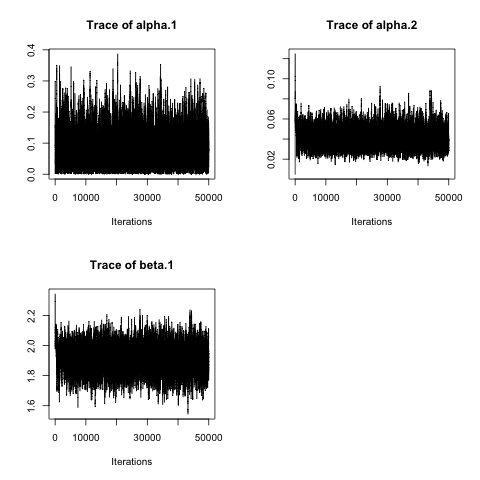
summary(mcmcout_M8, start = 1001)
plot(mcmcout_M8, partype = "parameter", density = FALSE )## Model: SI distance-based discrete-time ILM
## Method: Markov chain Monte Carlo (MCMC)
##
## Iterations = 1001:50000
## Thinning interval = 1
## Number of chains = 1
## Sample size per chain = 49000
##
## 1. Empirical mean and standard deviation for each variable,
## plus standard error of the mean:
##
## Mean SD Naive SE Time-series SE
## alpha.1 0.08383 0.05640 2.548e-04 0.0011732
## alpha.2 0.04127 0.01018 4.597e-05 0.0002205
## beta.1 1.90953 0.09091 4.107e-04 0.0018415
##
## 2. Quantiles for each variable:
##
## 2.5% 25% 50% 75% 97.5%
## alpha.1 0.005079 0.03986 0.07547 0.11606 0.21817
## alpha.2 0.024144 0.03398 0.04029 0.04758 0.06363
## beta.1 1.727576 1.84792 1.91001 1.97248 2.08330
We now turn to techniques that can be used for model comparison. This is done using the deviance information criterion (DIC) to compare the fit of different models via the epidic() function. So, we perform the MCMC analysis again without the susceptibility covariate, and then we use the epidic() function to calculate the DIC value for each model. The model with lowest DIC value is deemed to have the best fit under this criterion (after allowing for stochastic variation).
mcmcout_M9 <- epimcmc(out_cov,
    tmax = t_end, niter = 50000, sus.par.ini = 0.01,
    beta.ini = 2, pro.sus.var = 0.1, pro.beta.var = 0.5,
    prior.sus.dist = "uniform", prior.sus.par = c(0, 3),
    prior.beta.dist = "uniform", prior.beta.par = c(0, 10),
    adapt = TRUE, acc.rate = 0.5)

# to get DIC value for the two models (with and without the susceptibility covariate)
loglike1 <- epilike(object = out_cov, tmax = t_end, Sformula = ~A,
    sus.par = c(0.08806, 0.04421), beta = 1.96839)
loglike2 <- epilike(object = out_cov, tmax = t_end, sus.par = 0.735,
    beta = 1.554)

dic1 <- epidic(burnin = 10000, niter = 50000,
    LLchain = mcmcout_M8$Loglikelihood, LLpostmean = loglike1)
dic1

dic2 <- epidic(burnin = 10000, niter = 50000,
    LLchain = mcmcout_M9$Loglikelihood, LLpostmean = loglike2)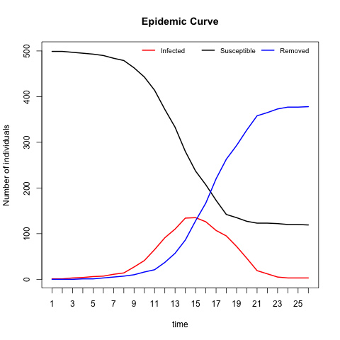
dic2Now we consider SIR network-based ILMs containing both susceptibility and transmissibility covariates. So, we start with generating an undirected binary contact network for a population of 500 individuals (for illustration).
# Load the EpiILM package
library("EpiILM")
set.seed(101)
# sample size
n <- 500
# Generating an undirected binary contact network:
contact <- matrix(0, n, n)
for(i in 1:(n-1)) {
	contact[i, ((i+1):n)] <- rbinom((n-i), 1, 0.05)
	contact[((i+1):n), i] <- contact[i, ((i+1):n)]
	}
Now, we generate two covariates to be used as susceptibility covariates. We will also use these covariates as transmissibility covariates. As we are now in an SIR framework, we have to set the infectious period for each infective. Here, we set the infectious period to be three time points for each infected individual. The rest of the analysis follows the general framework we saw for spatial ILMs.
# Generating the susceptibility and transmissibility covariates:
X1 <- round(rexp(n, 1/100))
X2 <- round(rgamma(n, 50, 0.5))
# Simulate epidemic form SIR network-based ILM
infp <- rep(3, n)
SIR.net <- epidata(type = "SIR", n = 500, tmax = 50,
    sus.par = c(0.003, 0.002), trans.par = c(0.0003, 0.0002),
    contact = contact, infperiod = infp,
    Sformula = ~ -1 + X1 + X2, Tformula = ~ -1 + X1 + X2)
# Epidemic curve for SIR.net
plot(SIR.net, plottype = "curve", curvetype = "complete")
# epimcmc function to estimate the model parameters:
t_end <- max(SIR.net$inftime)
prior_par <- matrix(rep(1, 4), ncol = 2, nrow = 2)
# This took 305.7 seconds on an Apple MacBook Pro with i5-core Intel 2.4 GHz
# processors with 8 GB of RAM.
mcmcout_SIR.net <- epimcmc(SIR.net, tmax = t_end, niter = 20000,
Sformula = ~-1 + X1 + X2, Tformula = ~-1 + X1 + X2,
sus.par.ini = c(0.003, 0.01), trans.par.ini = c(0.01, 0.01),
pro.sus.var = c(0.0, 0.1), pro.trans.var = c(0.1, 0.1),
prior.sus.dist = c("gamma", "gamma"), prior.trans.dist = c("gamma", "gamma"),
prior.sus.par = prior_par, prior.trans.par = prior_par,
adapt = TRUE, acc.rate = 0.5)
# Summary of MCMC results
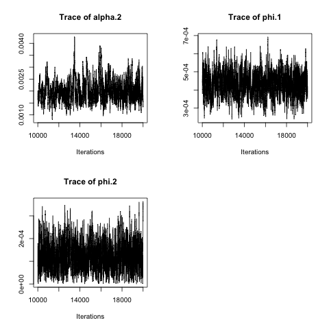
summary(mcmcout_SIR.net, start = 10001)
plot(mcmcout_SIR.net, partype = "parameter", start = 10001, density = FALSE)## Model: SIR network-based discrete-time ILM
## Method: Markov chain Monte Carlo (MCMC)
##
## Iterations = 10001:20000
## Thinning interval = 1
## Number of chains = 1
## Sample size per chain = 10000
##
## 1. Empirical mean and standard deviation for each variable,
## plus standard error of the mean:
##
## Mean SD Naive SE Time-series SE
## alpha.2 0.0020169 4.676e-04 4.676e-06 2.833e-05
## phi.1 0.0004338 6.791e-05 6.791e-07 3.189e-06
## phi.2 0.0001242 6.192e-05 6.192e-07 2.236e-06
##
## 2. Quantiles for each variable:
##
## 2.5% 25% 50% 75% 97.5%
## alpha.2 1.267e-03 0.0016953 0.0019510 0.0022695 0.0031048
## phi.1 3.067e-04 0.0003871 0.0004321 0.0004793 0.0005688
## phi.2 1.797e-05 0.0000792 0.0001187 0.0001641 0.0002588
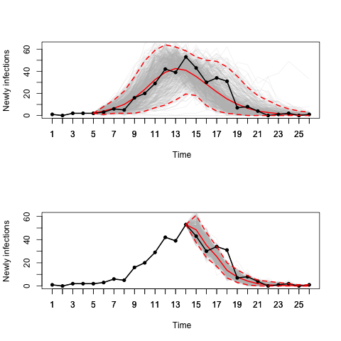
We can also consider forecasting from a fitted model. Here we see two examples, one uses data up to time point 5 to fit the model and then forecasts forward using a posterior predictive approach. The second does the same but using data up to time point 14 to fit the model before predicting forwards in time.
# Posterior predictive forecasting
# Posterior prediction starting from time point 5
pred.SIR.net.point.5 <- pred.epi(SIR.net, xx = mcmcout_SIR.net, tmin = 5,
    Sformula = ~-1 + X1 + X2, Tformula = ~-1 + X1 + X2,
    burnin = 1000, criterion = "newly infectious",
    n.samples = 500)

# Posterior prediction starting from time point 14
pred.SIR.net.point.8 <- pred.epi(SIR.net, xx = mcmcout_SIR.net, tmin = 14,
    Sformula = ~-1 + X1 + X2, Tformula = ~-1 + X1 + X2,
    burnin = 1000, criterion = "newly infectious",
    n.samples = 500)

# plot predictions:
par(mfrow = c(2,1))
plot(pred.SIR.net.point.5, col = "red", lwd = 2, pch = 19)
plot(pred.SIR.net.point.8, col = "red", lwd = 2, pch = 19)
Deardon, R., Brooks, S. P., Grenfell, B. T., Keeling, M. J., Tildesley, M. J., Savill, N. J., Shaw, D. J., and Woolhouse, M. E. (2010). Inference for individual level models of infectious diseases in large populations. Statistica Sinica, 20, 239-261.
- R - The Comprehensive R Archive Network
- Vineetha Warriyar K. V. - Author and Maintainer
- Waleed Almutiry - Author
- Rob Deardon - Author
This project is licensed under the GNU General Public License, version 3 - see the (http://www.r-project.org/Licenses/GPL-3) file for details.