MathBox is a computational graphing library. In simple use cases, it can elegantly draw 2D, 3D or 4D graphs, including points, vectors, labels, wireframes and shaded surfaces.
In more advanced use, data can be processed inside MathBox, compiled into GPU programs which can feed back into themselves. By combining shaders and render-to-texture effects, you can create sophisticated visual effects, including classic Winamp-style music visualizers.
You create MathBox scenes by composing a MathBox object tree, similar to HTML. Unlike HTML, the DOM is defined in JavaScript. This lets you freely mix the declarative model with custom expressions.
To show anything in MathBox, you need to establish four things:
- A camera that is looking at...
- A coordinate system which contains...
- Geometrical data represented via...
- A choice of shape to draw it as.
For example, a 2D rectangular view containing an array of points, drawn as a continuous line. Let's do that.
Download MathBox (ZIP). See README for more info.
Note: Open examples/empty.html in your text editor and browser to follow along. You can also use the JSBin, but you'll want to turn off "Auto-run" in the top right.
The default 3D camera starts out at [0, 0, 0] (i.e. X, Y, Z), right in the middle of our diagram. +Z goes out of the screen and -Z into the screen.
We insert our own camera and pull back its position 3 units to [0, 0, 3]. We also set proxy to true: this allows interactive camera controls to override our given position.
var camera = mathbox.camera({
  proxy: true,
  position: [0, 0, 3],
});
Our mathbox DOM now looks like:
<root>
  <camera proxy={true} position={[0, 0, 3]} />
</root>
Note: You can look at the state of the DOM at any time by doing mathbox.print().
The return value, camera, is a mathbox selection that points to the <camera /> element. This is similar to how jQuery selections work. You can also select elements with CSS selectors, e.g. finding our camera:
camera = mathbox.select('camera');Now we're going to set up a simple 2D cartesian coordinate system. We'll make it twice as wide as high.
var view = mathbox.cartesian({
  range: [[-2, 2], [-1, 1]],
  scale: [2, 1],
});
The range specifies the area we're looking at as an array of pairs, [-2, 2] in the X direction, [-1, 1] in the Y direction.
The scale specifies the projected size of the view, in this case [2, 1], i.e. 2 X units and 1 Y unit.
We'll immediately add two axes and a grid so we can finally see something:
view
  .axis({
    axis: 1,
    width: 3,
  })
  .axis({
    axis: 2,
    width: 3,
  })
  .grid({
    width: 2,
    divideX: 20,
    divideY: 10,
  });
You should see them appear in 50% gray, the default color, at the given widths. The DOM now looks like this:
<root>
  <camera proxy={true} position={[0, 0, 3]} />
  <cartesian range={[[-2, 2], [-1, 1]]} scale={[2, 1]}>
    <axis axis={1} width={3} />
    <axis axis={2} width={3} />
    <grid width={2} divideX={20} divideY={10} />
  </cartesian>
</root>
You could make your axes black by giving them a color: "black", either by adding the property above, or by setting it after the fact:
mathbox.select('axis').set('color', 'black');As the on-screen size of elements depends on the position of the camera, we can calibrate our units by setting the focus on the <root> to match the camera distance:
mathbox.set('focus', 3);Which gives us:
<root focus={3}>
  <camera proxy={true} position={[0, 0, 3]} />
  <cartesian range={[[-2, 2], [-1, 1]]} scale={[2, 1]}>
    <axis axis={1} width={3} color="black" />
    <axis axis={2} width={3} color="black" />
    <grid width={2} divideX={20} divideY={10} />
  </cartesian>
</root>
Note: You can use .get("prop")/.set("prop", value) to set individual properties, or use .get() and .set({ prop: value }) to change multiple properties at once.
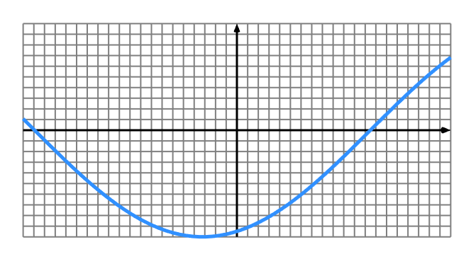
Now we'll draw a moving sine wave. First we create an interval, this is a 1D array, sampled over the cartesian view's range. It contains an expr, an expression to generate the data points.
We generate 64 points, each with two channels, i.e. X and Y values.
var data =
  view.interval({
    expr: function (emit, x, i, t) {
      emit(x, Math.sin(x + t));
    },
    length: 64,
    channels: 2,
  });
Here, x is the sampled X coordinate, i is the array index (0-63), and t is clock time in seconds, starting from 0. The use of emit is similar to returning a value. It is used to allow multiple values to be emitted very efficiently.
Once we have the data, we can draw it, by adding on a <line />:
var curve =
  view.line({
    width: 5,
    color: '#3090FF',
  });
Here we use an HTML hex color instead of a named color. CSS syntax like "rgb(255,128,53)" works too.
The DOM now looks like:
<root focus={3}>
  <camera proxy={true} position={[0, 0, 3]} />
  <cartesian range={[[-2, 2], [-1, 1]]} scale={[2, 1]}>
    <axis axis={1} width={3} color="black" />
    <axis axis={2} width={3} color="black" />
    <grid width={2} divideX={20} divideY={10} />
    <interval expr={(emit, x, i, t) => {
          emit(x, Math.sin(x + t));
        }} length={64} channels={2} />
    <line width={5} color="#3090FF" />
  </cartesian>
</root>The nice thing about separating data from shape is that you can draw the same data multiple ways. For example, add on <point /> to draw points as well:
var points =
  view.point({
    size: 8,
    color: '#3090FF',
  });
The different shapes available are documented in primitives.md. Points, lines and surfaces are pretty obvious and do what it says on the tin. e.g. Fill a 2D <area> will data and pass it to a <surface> to draw a solid triangle mesh.
For vectors, faces and strips though, the situation changes. To draw 64 vectors as arrows, you need 128 points: a start and end for each. Thus the data has to change. We set items to 2 and emit two points per iteration. We also add on a green <vector /> to draw the data:
var vector =
  view.interval({
    expr: function (emit, x, i, t) {
      emit(x, 0);
      emit(x, -Math.sin(x + t));
    },
    length: 64,
    channels: 2,
    items: 2,
  })
  .vector({
    end: true,
    width: 5,
    color: '#50A000',
});<root focus={3}>
<camera proxy={true} position={[0, 0, 3]} />
<cartesian range={[[-2, 2], [-1, 1]]} scale={[2, 1]}>
<axis axis={1} width={3} color="black" />
<axis axis={2} width={3} color="black" />
<grid width={2} divideX={20} divideY={10} />
<interval expr={(emit, x, i, t) => {
emit(x, Math.sin(x + t));
}} length={64} channels={2} />
<line width={5} color="#3090FF" />
<point size={8} color="#3090FF" />
<interval expr={(emit, x, i, t) => {
emit(x, 0);
emit(x, -Math.sin(x + t));
}} length={64} channels={2} items={2} />
<vector end={true} width={5} color="#50A000" />
</cartesian>
</root>Alternatively, you can also supply an array of data, either constant or changing, flat or nested. MathBox will iterate over it and emit it for you, picking up any live data. If your data does not change, you can set live: false to optimize.
Finally we'll label our coordinate system. First we need to establish a <scale />, which will divide our view into nice intervals.
var scale =
  view.scale({
    divide: 10,
  });
We can draw our scale as tick marks with <ticks />:
var ticks =
  view.ticks({
    width: 5,
    size: 15,
    color: 'black',
  });
Now we need to format our numbers into rasterized text:
var format =
  view.format({
    digits: 2,
    weight: 'bold',
  });
And finally draw the text as floating labels:
var labels =
  view.label({
    color: 'red',
    zIndex: 1,
  });
Here we apply zIndex similar to CSS to ensure the labels overlap in 2D rather than being placed in 3D. It specifies a layer index, with 0 being the default, and layers 1...n stacking on top. Negative zIndex is not allowed.
Note: Unlike CSS, large zIndex values are not recommended, as the higher the z-Index, the less depth resolution you have.
Finally we'll add on a little bit of animation by adding a <play /> block.
var play = mathbox.play({
  target: 'cartesian',
  pace: 5,
  to: 2,
  loop: true,
  script: [
    {props: {range: [[-2, 2], [-1, 1]]}},
    {props: {range: [[-4, 4], [-2, 2]]}},
    {props: {range: [[-2, 2], [-1, 1]]}},
  ]
});
Here script defines the keyframes we'll be animating through. We specify props will change, namely the range. We pass in the keyframes as an array, which will assign them to evenly spaced keyframes (0, 1, 2).
We set the pace of the animation to 5 seconds per step, tell it to play till keyframe time 2 and to loop afterwards.
<root focus={3}>
  <camera proxy={true} position={[0, 0, 3]} />
  <cartesian range={[[-2, 2], [-1, 1]]} scale={[2, 1]}>
    <axis axis={1} width={3} color="black" />
    <axis axis={2} width={3} color="black" />
    <grid width={2} divideX={20} divideY={10} />
    <interval expr={(emit, x, i, t) => {
          emit(x, Math.sin(x + t));
        }} length={64} channels={2} />
    <line width={5} color="#3090FF" />
    <point size={8} color="#3090FF" />
    <interval expr={(emit, x, i, t) => {
          emit(x, 0);
          emit(x, -Math.sin(x + t));
        }} length={64} channels={2} items={2} />
    <vector end={true} width={5} color="#50A000" />
    <scale divide={10} />
    <ticks width={5} size={15} color="black" />
    <format digits={2} weight="bold" />
    <label color="red" zIndex={1} />
  </cartesian>
  <play target="cartesian" to={2} loop={true} pace={5} script={[{props: {range: [[-2, 2], [-1, 1]]}}, {props: {range: [[-4, 4], [-2, 2]]}}, {props: {range: [[-2, 2], [-1, 1]]}}]} />
</root>
When you're done, you can do a mathbox.remove("*") to empty out the tree and start with a clean slate, or mathbox.select('cartesian > *').remove() to empty out the view only.
See examples/ for more ideas and examples/test for specific usage.