GMPE-estimation

This repository provides the MATLAB scripts used to estimate ground-motion prediction equations (GMPE) with spatial correlation. The scripts are produced as by-products of the following paper:

Ming, D., Huang, C., Peters, G.W., and Galasso, C. An advanced estimation algorithm for ground-motion models with spatial correlation. Bulletin of the Seismological Society of America, 2019.

This algorithm provides uncertainty quantifications (in terms of asympototic standard deviation) of all model parameters including the range parameter (i.e., lengthscale) in the spatial correlation function. This feature of the algorithm is particularly advantageous because the computed measurement of uncertainty can also be used to check statistical significance and improve model specification. The estimated GMPE can also be used by the prediction function in this repository for intensity measure (IM) predictions at unknown locations with associated predictive uncertainty.

General info

The current version of the estimation scripts can be used to estimate a generic GMPE as long as the mean function of the GMPE can be written in the following form:

where β₁, β₂, β₃,... are linear coefficients in the mean function of a GMPE, and g₁( · ; · ), g₂( · ; · ), g₂( · ; · ),... are basis functions of input data X and nonlinear coefficients γ in the mean function of a GMPE and are first order differentiable wrt nonlinear coefficients γ. One needs to rewrite his own GMPE mean function in this functional form before implementing the estimation algorithm.

The intra-event correlation can be represented by one of the following four correlation functions:

• No spatial correlation:

  

• Exponential:

  

• Matérn with ν=1.5:

  

• Squared exponential:

  

Contents

The repository currently contains the following items:

• Akkar2010.mat: the MATLAB data file that contains the model parameter estimates of b, τ and σ given by Akkar and Bommer (2010);
• Bg.m: the MATLAB function that computes the grident of design matrix wrt nonlinear coefficients in the ground-motion prediction function of Akkar and Bommer (2010);
• data.mat: the MATLAB data file that contains an example of ground-motion records as the inputs to scoring.m;
• design.m: the MATLAB function that gives the design matrix of the linear coefficients in the ground-motion prediction function of Akkar and Bommer (2010);
• eventfinder.m: the MATLAB function that extracts information of a specified event from the ground-motion database;
• generator.m: the MATLAB function that generates synthetic logarithmic intensity measures (IM).
• grid_data.mat: the MATLAB data file that contains the covariate information at prediction locations;
• Italyborder.mat: the MATLAB data file that contains the coordinates of the border of Italy;
• prediction.m: the MATLAB function that make linear predictions on the specified locations given the observations at recording sites;
• scoring.m: the MATLAB function that implements the Scoring estimation approach for GMPEs with spatial correlation;
• semivag.m: the MATLAB function that plots the empirical semivariogram together with the fitted theoretical semivariogram models;
• shakemap.m: the MATLAB function that draws the shake map based on the produced predictions.

Update log

07.08.2020

• scoring.m: extra argument gamma_cstr is added so user can define which nonlinear coefficients in the mean function of GMPE have positivity constraints; the algorithm can now also estimate GMPE with only linear coefficients in its mean function by setting arguments gamma0=[], f2=[], and gamma_cstr=[];
• generator.m: now can generate synthetic logarithmic intensity measures (IM) for GMPE with only linear coefficients in its mean function by setting argument gamma=[];
• semivag.m: now can plot empirical semivariograms for GMPE with only linear coefficients in its mean function;
• prediction.m: now can make linear predictions for GMPE with only linear coefficients in its mean function. It now also outputs predictive variances at the predictions locations that can be used as uncertainty measurements of predictions made by the estimated GMPE;
• Various bugs of the algorithm are fixed for cases where there are more than one nonlinear coefficients in the GMPE.

02.05.2019

• generator.m: inputs are changed to be consistent with those of the updated scoring.m;
• prediction.m: inputs are changed to be consistent with those of the updated scoring.m;
• scoring.m: inputs are changed so a generic GMPE can be implemented. The outputs are now stored in a single structure format;
• semivag.m: inputs are changed to be consistent with those of of the updated scoring.m;
• Bg.m and design.m are added.

A synthetic example

This example illustrates a step-by-step instruction on how to use the Scoring estimation approach to estimate a GMPE of Akkar and Bommer (2010) with exponential spatial correlation function based on a synthetic dataset of logarithmic PGA.

• Step 1 - Data preparation

  The GMPE proposed by Akkar and Bommer (2010) is given by:

which can be written in the general form presented in General Info section by setting β₀=b₁, β₁=b₂, β₂=b₃, β₃=b₄, β₄=b₅, β₅=b₇, β₆=b₈, β₇=b₉, β₈=b₁₀ and γ=b₆. We then need to define two functions:

• Function 1: a matrix-valued function that outputs the design matrix of linear coefficients. For this example, this function is coded as design.m;
• Function 2: a function that outputs a cell, in which each element contains a matrix (same dimension as the design matrix) of gridents (i.e., first order derivatives) of the design matrix wrt to each nonlinear coefficient in the mean function of the GMPE. For this example, this function is coded as Bg.m.

Note: Users only need to change these two functions to accommodate their own GMPE mean function form. More details on how to construct these two functions can be found in the comments of design.m and Bg.m.

Now we load and assign data required for the estimation.

%load data
load('data.mat')

%Assign data to covariates in the ground-motion prediction function given by Akkar and Bommer (2010).
x=[data.Mw,data.JB_dist,data.Ss,data.Sa,data.Fn,data.Fr];

%Assign data to covariates (lat and lon) required in the correlation function
w=[data.st_latitude,data.st_longitude];

%Set earthquake ID
id=data.event_id;

• Step 2 - Synthetic data generation

  To generate synthetic logarithmic IMs (PGA in this case), we need to decide the type of correlation function to, choose values of model parameters, and pick the number of synthetic logarithmic PGA dataset to be generated.

%Choose correlation function type ('No','Exp' or 'Matern1.5' or 'SExp')
cf='Exp';

%Assign parameter values given by Akkar and Bommer (2010)
%para(1:10) correspond to b, para(11) and para(12) correspond to tau and sigma, respectively
load('Akkar2010.mat')
para=Akkar2010; 
%linear coefficients
beta=[para(1:5),para(7:10)]'; 
%nonlinear coefficients. gamma should be specified as a column vector when there are more than one nonlinear coefficients
gamma=para(6); 
%Assign a value to the range parameter h in the exponential correlation function
h=11.5; 
theta=[para(11)^2;para(12)^2;h];

%Generate one set of log(IM) (i.e., log(PGA))
n=1;
y=generator(x,w,id,beta,gamma,theta,@design,n,cf);

• Step 3 - Estimation

  The estimation of GMPE is then can be implemented by executing the following scripts:

%Set the initial value for the nonlinear coefficients (b_6 in this example)
%(gamma0 should be specified as a column vector when there are more than one nonlinear coefficients)
gamma0=para(6)-1;

%Set initial values for the inter- and intraevent variances and the range parameter h
theta0=[para(11)^2-0.001,para(12)^2-0.01,h-2]';

%In this example, we perturb the parameter values used to generate synthetic data as the initial values for the estimation

%Set the tolerance level for the optimization algorithm
tol=0.0001;

%Set the confidence level (95% in this example) to be used to construct confidence intervals for the parameter estimators
cl=95;

%Set a binary vector that indicates which nonlinear coefficients have positivity constraints
%(although b_6 should be positive, it is in quadratic form and thus does not need to be constrained to be positive during the optimisation)
gamma_cstr=[0];

%Begin the estimation
output_syn=scoring(y,x,w,id,@design,@Bg,gamma0,theta0,tol,cl,cf,gamma_cstr);

%%%%%%%%%%%%COMMAND WINDOW OUTPUTS%%%%%%%%%%%%
  Iteration 0 Loglikelihood   107.7564
  Iteration 1 Loglikelihood   120.1908
  Iteration 2 Loglikelihood   120.3800
  Iteration 3 Loglikelihood   120.3845
  Iteration 4 Loglikelihood   120.3847
  Converged!
%%%%%%%%%%%%%%%%%%%%%%%%%%%%%%%%%%%%%%%%%%%%%%
Note: your outputs will differ from the above depending on your synthetic data. 

• Step 4 - Extraction of results

  The estimation results can be extracted from the output_syn variable:

  • InformationCriteria: the AIC and BIC values;
  • LogLikelihood: the log-likelihood value at convergence;
  • ParameterEstimates: the estimates of all model parameters;
  • StandardError: the asymptotic standard error estimates of ML estimators of model parameters;
  • ConfidenceInterval: the confidence intervals (95% in this example) of all model parameters.

A real data example

In this section, we demonstrate in a real data example on how to use the Scoring estimation approach to estimate the GMPE proposed by Akkar and Bommer (2010) with spatial correlation.

• Step 1 - Initial estimation

  In this step, we estimate the GMPE proposed by Akkar and Bommer (2010) without considering the spatial correlation. The results of this initial estimation will provide information to preliminarily estimate spatial correlation function in Step 2.

%load data
load('data.mat')

%Assign data to covariates in the ground-motion prediction function given by Akkar and Bommer (2010).
x=[data.Mw,data.JB_dist,data.Ss,data.Sa,data.Fn,data.Fr];

%Assign data to covariates (lat and lon) required in the correlation function
w=[data.st_latitude,data.st_longitude];

%Set earthquake ID
id=data.event_id;

%Log transform the PGAs and assign them to the dependent variable
y=log10(data.rotD50_pga);

%Choose correlation function type ('No','Exp' or 'Matern1.5' or 'SExp')
cf='No';

%Assign parameter values given by Akkar and Bommer (2010)
%para(1:10) correspond to b, para(11) and para(12) correspond to tau and sigma, respectively
load('Akkar2010.mat')
para=Akkar2010; 

%Set the initial value for the nonlinear coefficients (b_6 in this example) as given by Akkar and Bommer (2010)
gamma0=para(6);

%Set initial values for the inter- and intraevent variances as given by Akkar and Bommer (2010)
theta0=[para(11)^2,para(12)^2]';

%Set the tolerance level for the optimization algorithm
tol=0.0001;

%Set the confidence level (95% in this example) to be used to construct confidence intervals for the parameter estimators
cl=95;

%Set a binary vector that indicates which nonlinear coefficients have positivity constraints
%(although b_6 should be positive, it is in quadratic form and thus does not need to be constrained to be positive during the optimisation)
gamma_cstr=[0];

%Begin the estimation
output_ini=scoring(y,x,w,id,@design,@Bg,gamma0,theta0,tol,cl,cf,gamma_cstr);

%%%%%%%%%%%%COMMAND WINDOW OUTPUTS%%%%%%%%%%%%
  Iteration 0 Loglikelihood  -877.7142
  Iteration 1 Loglikelihood  -728.0676
  Iteration 2 Loglikelihood  -711.1419
  Iteration 3 Loglikelihood  -709.8849
  Iteration 4 Loglikelihood  -709.8144
  Iteration 5 Loglikelihood  -709.8132
  Iteration 6 Loglikelihood  -709.8132
  Converged!
%%%%%%%%%%%%%%%%%%%%%%%%%%%%%%%%%%%%%%%%%%%%%%

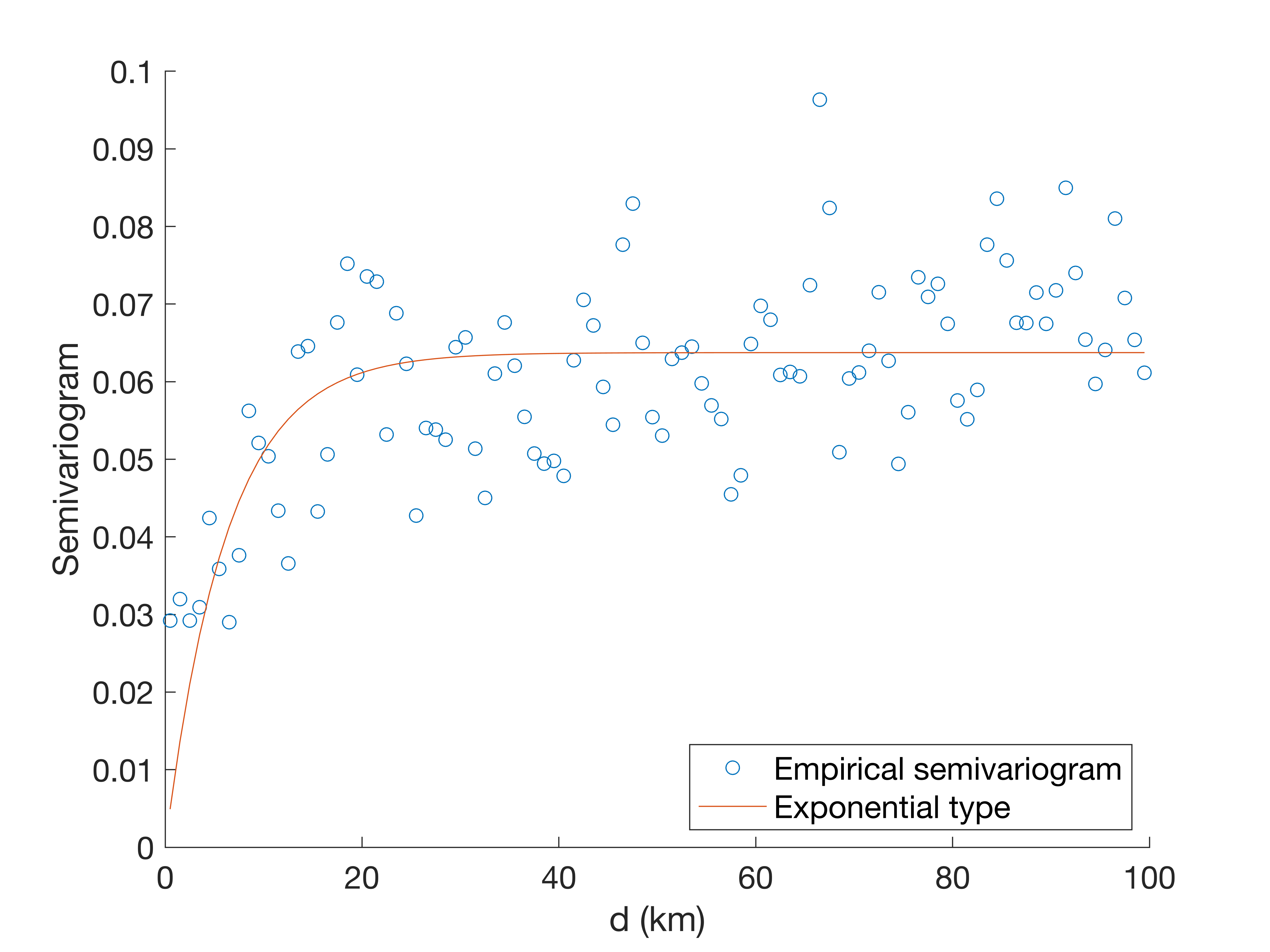
• Step 2 - Preliminary estimation of the range paramter

  In this step, we use the estimates obtained in Step 1 to obtain the preliminary estimate of the range parameter via the semivariogram.

%Set an initial value for the range parameter h
h0=40;

%Set the binwidth for the empirical semivariogram
deltah=0.5;

%Plot empirical semivariogram with the fitted exponential semivariograms
[varcomponents_exp,semivar]=semivag(y,x,w,id,output_ini,@design,h0,deltah,'Exp');

This will produce the following figure:

• Step 3 - Estimation

  In this step, we use the preliminary estimate of h obtained in Step 2 to implement the one-stage estimation algorithm.

%Set initial value for the nonlinear coefficient b_6 as the one estimated from Step 1 
gamma0=output_ini.ParameterEstimates.gamma;

%Set initial value for the interevent variance tau^2 as the one estimated from Step 1
tau20=output_ini.ParameterEstimates.theta(1);

%Set initial values for the intraevent variance sigma^2 and the range parameter h as the ones estimated from Step 2
sigma20_exp=varcomponents_exp(1);
h0_exp=varcomponents_exp(2);

%Combine initial values
gamma0_exp=gamma0;
theta0_exp=[tau20;sigma20_exp;h0_exp];

%Begin estimation
output_real=scoring(y,x,w,id,@design,@Bg,gamma0_exp,theta0_exp,tol,cl,'Exp',gamma_cstr);

%%%%%%%%%%%%COMMAND WINDOW OUTPUTS%%%%%%%%%%%%
      .             .             .
      .             .             .
      .             .             .
  Iteration 32 Loglikelihood  -675.1151
  Iteration 33 Loglikelihood  -675.1149
  Iteration 34 Loglikelihood  -675.1147
  Iteration 35 Loglikelihood  -675.1146
  Iteration 36 Loglikelihood  -675.1144
  Iteration 37 Loglikelihood  -675.1143
  Converged!
%%%%%%%%%%%%%%%%%%%%%%%%%%%%%%%%%%%%%%%%%%%%%%

Step 1 to 3 can be repeated for other choices of correlation functions, e.g., Matérn with ν=1.5 and squared exponential. However, the preliminary estimate of the range parameter obtained in Step 2 can be very biased as demonstrated in the paper, giving an unreasonable initial value to h, which in turn will cause ill-conditioning problems (for the squared exponential type, particularly) to the estimation algorithm. In such case, users are suggested to try a smaller initial value for h and re-run the estimation algorithm.

Though we will not go through in this example, users of the scripts are suggested to always check the statistical significances of model parameters via the confidence intervals produced by the estimation algorithm. This will help users decide whether some varaibles need to be removed, whether the model should be modified, whether more data are required to improve the statistical significance, etc. For example, in this real data case the magnitude and fault types are not statistically significant. This is because the information of the magnitude and fault types are given per event rather than per record, providing insufficient evidences to show they are statistically siginificant. Therefore, more events should be included in the training data. However, to prevent the curse of dimensionality, it might be a good idea to only include events with small numbers of records.

• Step 4 - Prediction

  In this step, we show how to draw a shake map for a given event based on the GMPE estimated in Step 3.

%Define the event under consideration
eventid='IT-1997-0137';

%Extract information of the event from the ground-motion database
[y_event,x_event,w_event]=eventfinder(eventid,id,y,x,w);

%load information at grid points (i.e., prediction locations)
load('grid_data.mat')

%Assign data to covariates in the ground-motion prediction function given by Akkar and Bommer (2010).
u_event=[grid_data.Mw,grid_data.JB_dist,grid_data.Ss,grid_data.Sa,grid_data.Fn,grid_data.Fr];

%Assign data to covariates (lat and lon) required in the correlation function
v_event=[grid_data.st_latitude,grid_data.st_longitude];

%Make predictions on grid points
[z_hat_exp,v_hat_exp]=prediction(y_event,x_event,u_event,w_event,v_event,output_real,@design,'Exp','off');

%load event map info
load('Italyborder.mat')

%Define the region of the shakemap
latRange=[40.68,45.18];
lonRang=[10.68,15.18];

%Draw the shake map without the log-scaled color (0) bar
lim=[min(z_hat_exp),max(z_hat_exp)];
f=shakemap(latRange,lonRang,Italyborder,w_event,v_event,z_hat_exp,0,lim);
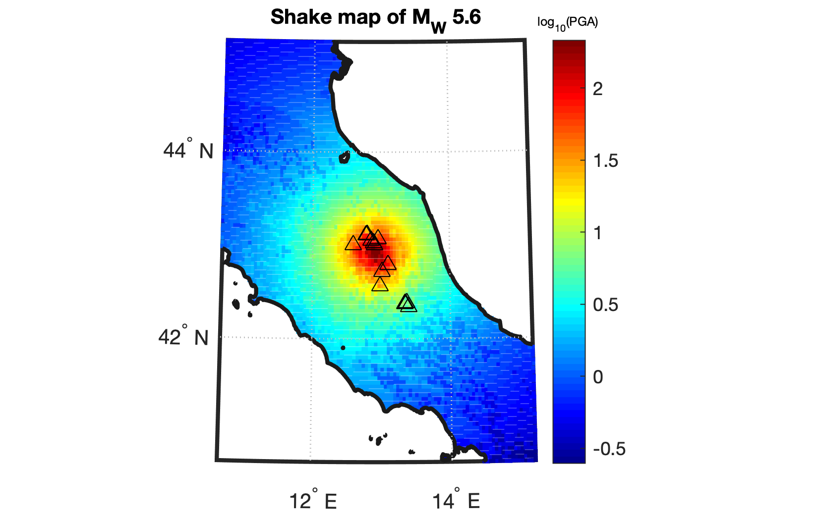
title('Shake map of M_W 5.6','fontsize',10);
hcb=colorbar;
title(hcb,'log_{10}(PGA)','fontsize',6);

The produced shake map in terms of log₁₀(PGA) is shown below, where the triangles are recording sites.

One can also plot the shake map in terms of PGA by:

%Make predictions on grid points and set the base to '10'
[z_hat_exp_delog,v_hat_exp_delog]=prediction(y_event,x_event,u_event,w_event,v_event,output_real,@design,'Exp','10');
%Draw the shakemap with log-scaled (1) color bar
lim=[min(z_hat_exp_delog),max(z_hat_exp_delog)];
f=shakemap(latRange,lonRang,Italyborder,w_event,v_event,z_hat_exp_delog,1,lim);
title('Shake map of M_W 5.6','fontsize',10);
hcb=colorbar;
title(hcb,'PGA (cm/s^2)','fontsize',6);

The resulting shake map is shown below, where the triangles are recording sites.

Note that user can use v_hat_exp or v_hat_exp_delog as the measurements of predictive uncertainty on grid points.

Built with

The scripts are built under MATLAB version R2018a.

License

The scripts are licensed under the GNU General Public License v3.0 - see the LICENSE file for details.

Contact

Please feel free to email me with any questions:

Deyu Ming (deyu.ming.16@ucl.ac.uk).