50 Must-Know Cluster Analysis Interview Questions

You can also find all 50 answers here 👉 Devinterview.io - Cluster Analysis

1. What is cluster analysis in the context of machine learning?

Cluster analysis groups data into clusters based on their similarity. This unsupervised learning technique aims to segment datasets, making it easier for machines to recognize patterns, make predictions, and categorize data points.

Key Concepts

• Similarity Measure: Systems quantify the likeness between data points using metrics such as Euclidean distance or Pearson correlation coefficient.

• Centroid: Each cluster in k-means has a central point (centroid), often positioned as the mean of the cluster's data points.

• Distance Matrix: Techniques like hierarchical clustering use a distance matrix to determine which data points or clusters are most alike.

Applications

• Recommendation Systems: Clustered user preferences inform personalized recommendations.

• Image Segmentation: Grouping elements in an image to distinguish objects or simplify depiction.

• Anomaly Detection: Detecting outliers by referencing their deviation from typical clusters.

• Genomic Sequence Analysis: Identifying genetic patterns or disease risks for precision medicine.

Limitations

• Dimensionality: Its effectiveness can decrease in high-dimensional spaces.

• Scalability: Some clustering methods are computationally intensive for large datasets.

• Parameter Settings: Appropriate parameter selection can be challenging without prior knowledge of the dataset.

• Data Scaling Dependency: Performance might be skewed if features aren't uniformly scaled.

2. Can you explain the difference between supervised and unsupervised learning with respect to cluster analysis?

Supervised learning typically involves labeled data, in which both features and target values are provided during training. Algorithms learn to predict target values by finding patterns within this labeled data.

On the other hand, unsupervised learning uses unlabeled data, where only the input features are available. Algorithms operating in this mode look for hidden structure within this data, typically without any specific target in mind.

Relationship to Clustering

• Supervised learning tasks often do not involve cluster analysis directly. However, models trained using labeled data can sometimes be used to identify underlying clusters within the data.

• Unsupervised learning, and specifically cluster analysis, is designed to partition data into meaningful groups based solely on the provided feature set.

Example Applications:

• Supervised Learning: Tasks like email classification as "spam" or "not spam" are classic examples. The model is trained on labeled emails.
• Unsupervised Learning: It is useful in cases such as customer segmentation for personalized marketing, where we want to identify distinct groups of customers based on their behavior without prior labeled categories.

Key Concepts

In the context of clustering:

• Supervised Learning typically hinges on methods aimed at predicting numerical values or categorical labels.
• Unsupervised Learning serves to uncover patterns or structures that are latent or inherent within the data.

In other words, supervised tasks typically involve target prediction, whereas unsupervised learning centers around knowledge discovery.

The Dynamics of Data

• Supervised Learning: The training data must be previously labeled, and it's the algorithm's job to learn the relationship between the provided features and the known labels or targets.

• Unsupervised Learning: The algorithm explores the data on its own, without any pre-existing knowledge of labels or categories. Instead, it looks for inherent structures or patterns. This exploration often takes the form of tasks like density estimation, dimensionality reduction, association rule mining, and, of course, cluster analysis.

Complexity and Interpretability

• Supervised Learning: The potential complexity of the relationships to be learned in the data is influenced by the label set provided during training. For example, in classification tasks where there might be an overlap between classes or non-linear decision boundaries, the underlying relationship might be complex, requiring sophisticated models. However, with the presence of well-defined labels, the interpretation of these models tends to be more straightforward.

• Unsupervised Learning: The relationships to be identified are based solely on the input features' structure and strength. As a result of the absence of provided labels, this setting often necessitates more in-depth exploration of the results. The interpretability of these models can sometimes be more challenging due to the intriguing, yet potentially vague, nature of the discovered patterns or clusters. Such vagueness can arise from the absence of an explicit ground truth with which to compare, potentially leading to differing cluster solutions depending on, for example, specific initializations in certain unsupervised techniques.

Practical Considerations

• Balance and Integration: Utilizing elements of both supervised and unsupervised learning can provide insightful results. For example, one might incorporate cluster structures identified through unsupervised methods as features for a subsequent supervised task, thereby leveraging the strengths of both paradigms.

• Resource and Data Availability: The need for labeled data in supervised learning can be a potential limitation, as obtaining such data can sometimes be costly or time-consuming. Unsupervised learning might be favored when labeled data are scarce. Furthermore, access to high-quality labels can be a potential concern, especially when such labels might be subjective or uncertain, potentially affecting the modeling performance in a supervised setting.

• Quality of Insight: While supervised learning can provide a direct link between the provided features and the targeted labels, the potential knowledge that can be inferred from unsupervised learning, such as the identification of previously unknown similarities or relationships, can offer a unique type of understanding.

3. What are some common use cases for cluster analysis?

Cluster analysis is versatile and finds application across multiple domains.

Common Use Cases

1. Customer Segmentation

   Identify market segments for targeted advertising and tailored product offers.

2. Anomaly Detection

   Uncover outliers or abnormalities in data, especially useful for fraud detection.

3. Recommendation Systems

   Group different items or content based on their similarities, allowing for personalized recommendations.

4. Image Segmentation

   Break down images into smaller regions or objects, which can assist in various image-related tasks, such as in medical imaging.

5. Text Categorization

   Automatically classify text documents into different clusters, aiding in tasks such as news categorization.

6. Search Result Grouping

   Cluster search results to offer more organized and diverse result sets to users.

7. Time Series Clustering

   Discover patterns and trends in time series data, useful in financial markets and forecasting.

8. Social Network Analysis

   Uncover groups or communities in social networks, enabling targeted advertising or campaign strategies.

9. Biological Data Analysis

   Analyze biological data, such as gene expression levels, to identify groups or patterns in genetic data.

10. Astronomical Data Analysis

    Group celestial objects based on their features, aiding in star or galaxy classification.

11. Insurance Premium Calculation

    Use clustering to categorize policyholders or claimants, informing the formulation of risk assessment and premium calculations.

12. Managing Inventory

Group inventory based on demand patterns or sales compatibility, aiding in optimized stock management.

13. Cybersecurity

    Identify patterns in network traffic to detect potential cyber threats or attacks.

14. Machine Fault Diagnosis

Utilize sensor data to categorize and predict potential equipment or machine failures.

15. Data Preprocessing

    As a preprocessing step for other tasks, such as in feature engineering.

16. Vocabulary Building in NLP

    Form groups of words for building a better vocabulary for NLP tasks.

4. How does cluster analysis help in data segmentation?

Data segmentation is the process of dividing a dataset into distinct groups based on shared characteristics. Cluster analysis accomplishes this task and benefits various domains, from customer segmentation to automatic tagging in image recognition.

Data Segmentation and Cluster Analysis

• Intent: Describe the role and utility of cluster analysis in data segmentation.
• Methods: Examples, Visuals (if applicable)

Segmentation Example: Food Delivery

In a food delivery dataset, let's assume the goal is to segment customers based on behavioral patterns for personalized targeting.

Clusters obtained through k-means or another method could include:

• "Busy Professionals" who make frequent, small-portion orders during weekdays.
• "Occasional Foodies" who place larger orders on weekends.
• "Health Enthusiasts" who consistently order from fitness-oriented restaurants.

Segmentation Example: Image Recognition

In the context of image recognition, cluster analysis, especially through methods like k-means, can be utilized to automatically tag and organize images.

If we consider a database of wildlife images, cluster analysis can group together images of the same species based on visual features. This can be immensely useful for accurate tagging and retrieval.

5. What are the main challenges associated with clustering high-dimensional data?

Clustering high-dimensional data poses unique challenges that traditional methods designed for low-dimensional data may struggle to address. Let's take a look at these challenges:

Challenges of High-Dimensional Data

• Curse of Dimensionality: As the number of dimensions increases, the data becomes increasingly sparse, leading to unreliable distance metrics. This issue impairs the ability of distance-based clustering algorithms such as $k$-means and hierarchical clustering.

• Degradation of Euclidean Distance: While the Euclidean distance measure is intuitive and widely used, it often becomes less meaningful in high-dimensional spaces. The "flattening effect" makes points seem equidistant, and the influence of this effect grows with dimensionality.

• Clustering Quality Deterioration: High-dimensional data can result in suboptimal clustering solutions, reducing the overall quality and interpretability of clusters.

• Loss of Discriminative Power: With a countless number of potential projections in high-dimensional space, traditional visual inspection methods, like scatterplots, lose their effectiveness. Not all clusters are guaranteed to be adjacent in any two-dimensional projection, leading to the "small cluster" and "compact cluster" problems.

• Increased Computational Demands: As the feature space expands, the computational cost of clustering algorithms, particularly those dependent on pairwise distance computations, escalates significantly.

• More Susceptibility to Noise and Outliers: High-dimensional spaces are inherently more susceptible to noise, which can affect the validity of the cluster structure. The influence of outliers can be magnified as well.

• Dimension Reduction Challenges: Pre-processing high-dimensional data via dimension reduction may not always be straightforward, especially when it involves preserving certain characteristics important for clustering.

• Interpretation and Communication Hurdles: It is more complex to visually or conceptually convey the nature of high-dimensional clusters and their defining features.

• Feature Selection Complexity: In high-dimensional data, identifying which features are most relevant for the clustering task can be a challenge in itself.

Considering these challenges, selecting the most fitting clustering approach for high-dimensional datasets is crucial. Algorithms like DBSCAN, which are less affected by the curse of dimensionality, or density-based methods like OPTICS or HDBSCAN, are often recommended. Also, model-based clustering methods can show more robustness in high-dimensional settings.

6. Discuss the importance of scaling and normalization in cluster analysis.

Scaling and Normalization influence the outcome of a clustering analysis. Clustering is often sensitive to the scaling of the data. Therefore, it's essential to get the correct scale to ensure that the model converges accurately.

The Role of Distances

• Euclidean and Manhattan Distances: These metrics are sensitive to varying scales. For example, a one-unit change in a dimension with a larger scale attribute would overshadow multiple units of change in a smaller scale attribute.

• Cosine Similarity: This measure is more robust to scale disparities as it focuses on angles, not magnitudes.

Impact on Algorithms

• K-Means: This method tries to minimize the sum of squared distances within clusters. Given its use of Euclidean distance, it is sensitive to scaling.

• Hierarchical Clustering: The choice of distance metric (e.g., Euclidean, Manhattan, or others) influences the method's performance with scaled data.

• DBSCAN: This approach uses a distance parameter to identify neighbor points for core point determination. Scaled data affects this distance, thereby impacting core point identification and the clustering outcome.

Consequences of Unscaled Data

Without scaling or standardizing data, attributes whose magnitudes are orders of magnitude greater could disproportionately influence the results, leading to ineffective clusters.

Techniques for Scaling

• Min-Max Scaling: It transforms data within a fixed range (usually 0 to 1).
• Z-Score Standardization: This ensures transformed data has a mean of 0 and a standard deviation of 1.
• Robust Scaling: It's similar to Z-score, but uses the median and interquartile range, making it less sensitive to outliers.

Code Example: Unchecked Data Scaling's Impact on K-Means

Here is the Python code:

from sklearn.cluster import KMeans
import numpy as np

# Generating random data with two features
np.random.seed(0)
X = np.random.rand(100, 2)

# Doubling the values of the first feature
X[:, 0] *= 2

# Fit and Predict with unscaled data
kmeans = KMeans(n_clusters=3, random_state=0).fit(X)
predictions = kmeans.predict(X)

# Visualizing the clusters
plt.scatter(X[:, 0], X[:, 1], c=predictions, cmap='viridis')
plt.scatter(kmeans.cluster_centers_[:, 0], kmeans.cluster_centers_[:, 1], marker='*', s=300, c='r')
plt.show()

In this code, the first feature has been artificially doubled. Without scaling, K-Means would be biased toward this feature, even though both features should be equally relevant in this scenario.

7. How would you determine the number of clusters in a dataset?

Determining the optimal number of clusters in a dataset is a crucial step in most clustering techniques. Several methods can provide guidance in this regard.

Methods for Estimating Clusters

1. Visual Inspection: Plot the data and visually identify clusters. While this is subjective, it allows for quick insights.

2. Elbow Method: Compute the sum of square distances from each data point to the centroid of its assigned cluster. Plot these values for a range of cluster counts. The "elbow" point on the plot represents an optimal number of clusters, where the sum of square distances levels off.

3. Silhouette Score: Evaluate the quality of clusters by measuring how similar an object is to its own cluster (cohesion) compared to other clusters (separation). The silhouette score ranges from -1 to 1, with higher values indicating better-defined clusters.

4. Gap Statistic: Compare within-cluster variation for different numbers of clusters with that of a random data distribution. Using the "gap" between the two metrics, this method identifies an optimal number of clusters.

5. Cross-Validation Approach: Integrate cluster analysis with cross-validation to select the number of clusters that best fits the workflow.

6. Information Criteria Methods: Use statistical techniques to measure the trade-off between model fit and the number of parameters in the model.

7. Bootstrap: Create multiple datasets from the original one and run clustering algorithms on each. By analyzing the variability across these datasets, the "best" number of clusters can be estimated.

8. Hierarchical Clustering Dendrogram: Cut the tree at different heights and evaluate cluster quality to identify the optimal number of clusters.

9. Density-Based Clustering: Techniques such as DBSCAN do not explicitly require a predefined number of clusters. They can still provide valuable insights in terms of local neighborhood densities.

10. Model Specific Methods: Some clustering algorithms may have built-in methods to determine the optimal number of clusters, like the Gaussian Mixture Model through the Bayesian Information Criterion (BIC).

8. What is the silhouette coefficient, and how is it used in assessing clustering performance?

The silhouette coefficient is a technique used to evaluate the robustness of a clustering solution by measuring the proximity of data points to both their own clusters and other clusters. It provides a measure of how well each data point lies within its assigned cluster.

Calculation

The silhouette coefficient of a data point, $i$, is denoted as $s(i)$, and is calculated using the following formula:

$$ s(i) = \frac{b(i) - a(i)}{\max(a(i), b(i))} $$

where:

• $a(i)$: The average distance of data point $i$ to all other points in the same cluster.
• $b(i)$: The average distance of data point $i$ to all points in the nearest cluster (other than the one to which $i$ belongs).

The silhouette coefficient for an entire dataset is the mean of the silhouette coefficients for individual data points, ranging from -1 to 1.

Interpreting Silhouette Coefficients

• Close to 1: Data points are well-matched to the clusters they are assigned to, indicating a high-quality clustering result.
• Close to -1: Data points might have been assigned to the wrong cluster.
• Around 0: The data point is on or near the decision boundary between two neighboring clusters.

Python Example: Silhouette Coefficient

Here is the Python code:

from sklearn.datasets import make_blobs
from sklearn.cluster import KMeans
from sklearn.metrics import silhouette_samples, silhouette_score
import matplotlib.pyplot as plt
import numpy as np

# Generate sample data
X, _ = make_blobs(n_samples=300, centers=4, cluster_std=1, center_box=(-10, 10), random_state=1)

# Calculate the silhouette score for different numbers of clusters
range_n_clusters = [2, 3, 4, 5, 6]
for n_clusters in range_n_clusters:
    # Initialize the clusterer with n_clusters value and a random generator
    clusterer = KMeans(n_clusters=n_clusters, random_state=10)
    cluster_labels = clusterer.fit_predict(X)
    # Compute the average silhouette score
    silhouette_avg = silhouette_score(X, cluster_labels)
    print(f"For n_clusters = {n_clusters}, the average silhouette score is {silhouette_avg}")
    
    # Calculate the silhouette scores of each individual data point
    sample_silhouette_values = silhouette_samples(X, cluster_labels)
    y_lower = 10
    for i in range(n_clusters):
        # Aggregate the silhouette scores for samples belonging to the same cluster
        ith_cluster_silhouette_values = sample_silhouette_values[cluster_labels == i]
        ith_cluster_silhouette_values.sort()
        size_cluster_i = ith_cluster_silhouette_values.shape[0]
        y_upper = y_lower + size_cluster_i
        color = plt.cm.nipy_spectral(float(i) / n_clusters)
        plt.fill_betweenx(np.arange(y_lower, y_upper),
                          0, ith_cluster_silhouette_values, facecolor=color, edgecolor=color, alpha=0.7)
        plt.text(-0.05, y_lower + 0.5 * size_cluster_i, str(i))
        y_lower = y_upper + 10  # Add 10 for the next cluster
plt.title("Silhouette plot for various clusters")
plt.xlabel("Silhouette coefficient values")
plt.ylabel("Cluster label")
plt.show()

9. Explain the difference between hard and soft clustering.

Clustering is an unsupervised learning technique used to group similar data points. There are two primary methods for clustering: hard clustering and soft clustering.

Hard Clustering

In Hard Clustering, each data point either belongs to a single cluster or no cluster at all. It's a discrete assignment.

Example: K-means

Soft Clustering

Soft Clustering, on the other hand, allows for a data point to belong to multiple clusters with varying degrees of membership, usually expressed as probabilities.

It's more of a continuous assignment of membership.

Example: Expectation-Maximization (EM) algorithm, Gaussian Mixture Models (GMM)

10. Can you describe the K-means clustering algorithm and its limitations?

K-means is among the most popular clustering algorithms for its ease of use and efficiency. However, it does have some limitations.

Algorithm Steps

1. Initialization: Randomly select K centroid points from the data.
2. Assignment: Each data point is assigned to the nearest centroid.
3. Update: Recalculate the centroid of each cluster as the mean of all its members.
4. Convergence Check: Iterate steps 2 and 3 until the centroids stabilize, or the assignments remain unchanged for a specified number of iterations.

The algorithm aims to minimize the within-cluster sum of squares (WCSS), often visualized using the Elbow method.

Code Example: K-means Algorithm

Here is the Python code:

from sklearn.cluster import KMeans
# Assuming X is the data matrix
kmeans = KMeans(n_clusters=3, random_state=42).fit(X)

Limitations of K-means

• Sensitivity to Initial Centroid Choice: Starting with different initial centroids can lead to distinct final clusters.

• Assumptions on Cluster Shape: K-means can struggle with non-globular, overlapping, or elongated clusters.

• Challenge with Outliers: K-means is highly sensitive to outliers.

• Lack of Flexibility in Cluster Size and Shape: The predefined K can be suboptimal, leading to poorly defined or missed clusters.

• Need for Data Preprocessing:

  • Sensitive to feature scaling due to its distance-based nature.
  • A priori feature selection may be necessary.

• Sensitivity to Noisy Data: Outliers and irregular noise can distort the cluster assignments.

• Disparate Cluster Sizes: Larger and spread-out clusters can dominate the overall WCSS, resulting in uneven representation.

• Metric Dependence: The choice of distance metric can impact the clustering.

• Convergence Bracketing: Early termination based on the "no change" in assignments can be sensitive to the chosen criteria.

11. How does hierarchical clustering differ from K-means?

Hierarchical Clustering and the K-Means algorithm are both techniques for unsupervised learning, but they differ significantly in several critical aspects.

Key Distinctions

Methodology

• K-Means divides the dataset into pre-determined $k$ clusters. Data points are iteratively reassigned to the nearest cluster center until little to no change occurs.
• Hierarchical Clustering does not require a set number of clusters. It builds a tree or dendrogram to represent the arrangement of clusters and enables different strategies for cluster extraction.

Initiation and Sensitivity

• K-Means is significantly influenced by the choice of initial cluster centers. The outcome may vary with different starting configurations.
• Hierarchical Clustering does not rely on initializations and has lower sensitivity to outliers due to its merge-divide strategy.

Execution Order

• While K-Means is an iterative process, initializing cluster centers at each iteration, Hierarchical Clustering type can utilize a "divisive" (top-down) or "agglomerative" (bottom-up) approach.
  • In agglomerative, each data point starts as its cluster and, in each step, the two closest clusters are merged till one or $k$ clusters are left.
  • In divisive, all data points begin in one cluster, and the cluster is then successively divided into smaller, more specific clusters till a single observation or $k$ clusters are left.

Inference Strategy

• K-Means: An instance is assigned to the nearest cluster center, and the overall process aims to minimize the sum of squares.
• Hierarchical Clustering: This method allows several ways to infer clusters. For instance, to decide the number of clusters from the dendrogram, one can choose a defined cut-off point where the vertical line passes through the tallest unbroken line.

Visual Output

• K-Means: Visualizing clusters can be done in $2$ or $3$ dimensions using scatter plots. However, the 'essence' of clusters visually extracted may vary based on the viewpoint.
• Hierarchical Clustering: A dendrogram is an invaluable visual representation that provides a quick overview of potential cluster counts and how individual instances group and ungroup.

12. What is the role of the distance metric in clustering, and how do different metrics affect the result?

The selection of an appropriate distance metric is vital in ensuring the quality of a clustering algorithm. Metrics influence the geometry of cluster shapes and can significantly impact the clustering result.

Core Metrics

1. Euclidean Distance: $L2$ Norm is sensitive to scale and can under-perform with high-dimensional or mixed-variance data. Most widely used.

$$ d(\mathbf{p}, \mathbf{q}) = \sqrt{\sum_{i=1}^{n}(q_i - p_i)^2} $$

3. Manhattan Distance: Useful for highly dimensional data due to its scale-invariance. The length of a path between points is the sum of the absolute differences of their coordinates.

$$ d(\mathbf{p}, \mathbf{q}) = \sum_{i=1}^{n} |q_i - p_i| $$

4. Minkowski Distance: When $p = 1$, this is equivalent to Manhattan distance; when $p = 2$, it's the same as Euclidean. This metric serves as a unifying framework for other distance measures.

$$ d(x, y) = \left( \sum_{i=1}^{n} |x_i - y_i|^p \right)^{\frac{1}{p}} $$

Visual Comparison

Specialized Metrics

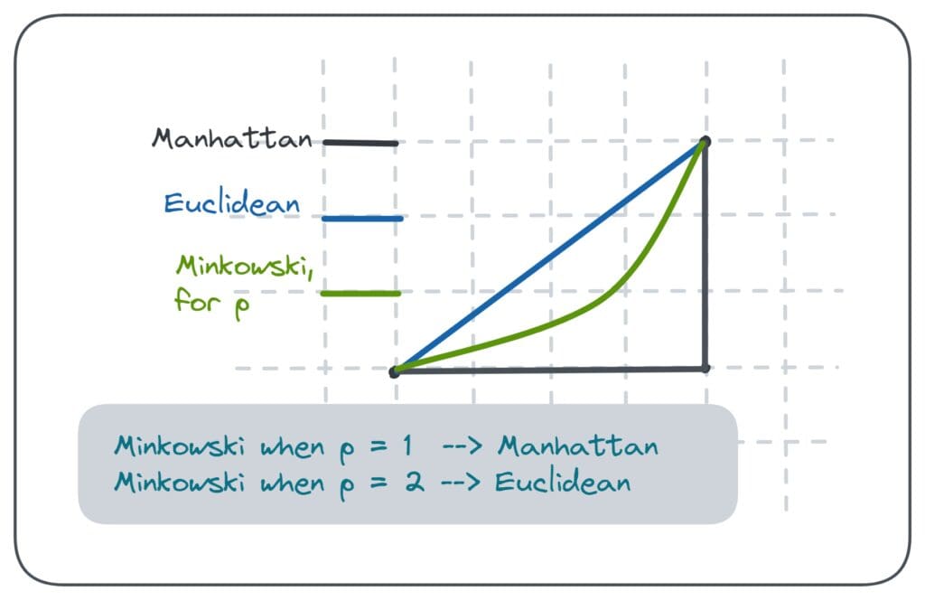
1. Mahalanobis Distance: It's a measure of the distance between a point and a distribution, taking into account the variance of the data. This can be especially useful when data dimensions are not independent. Mahalanobis distance reduces to the standard Euclidean distance when the covariance matrix is the identity matrix.

$$ d(\mathbf{p}, \mathbf{q}) = \sqrt{(\mathbf{p} - \mathbf{q})^T \mathbf{S}^{-1} (\mathbf{p} - \mathbf{q})} $$

2. Cosine Similarity: Rather than being a real distance metric, this is a similarity measure. It quantifies the similarity of two vectors based on the angle between them, being immune to their magnitudes. The angle between two vectors is used to compute the dot product, resulting in a value between -1 and 1. This measure is often employed in text mining, document clustering, and recommendation systems.

$$ \text{Cosine Similarity} = \frac{\mathbf{A} \cdot \mathbf{B}}{||\mathbf{A}|| ||\mathbf{B}||} = \frac{\sum_{i=1}^{n} A_i B_i}{\sqrt{\sum_{i=1}^{n} A_i^2} \sqrt{\sum_{i=1}^{n} B_i^2}} $$

13. Explain the basic idea behind DBSCAN (Density-Based Spatial Clustering of Applications with Noise).

DBSCAN (Density-Based Spatial Clustering of Applications with Noise) offers several advantages over k-means, especially for datasets with varying densities or noise.

Core Concepts

Epsilon-Neighborhood ($N_{\epsilon}$)

For a point $P$ in the dataset, its $N_{\epsilon}$ is the set of points within an epsilon (ε) distance from it.

$$ N_{\epsilon}(P) = {Q \text{ in dataset} | \text{dist}(P,Q) \le \epsilon} $$

MinPts

A minimum number of points (MinPts) is a specified parameter for DBSCAN indicating the minimum number of points needed within an epsilon-neighborhood for a point to be considered a core point.

Core, Border, and Noise Points

• Core point (P): A point with at least MinPts points in its epsilon-neighborhood.
• Border point (B): A point that is not a core point but is reachable from a core point.
• Noise point (N): A point that is neither a core point nor directly reachable from a core point.

Key Steps

1. Select Initial Point: A random, unvisited point is chosen.

2. Expand Neighbor: The algorithm forms a cluster by recursively visiting all the points in the MinPts neighborhood of the current point.

3. Validate: If the current point is a core point, all of its neighbors are added to the cluster. If not a core point, it is labeled a noise or border point, and the cluster formation process for the current branch is finished.

4. Explore New Branches: If a neighbor of the current point is a core point, the algorithm begins expanding the cluster from that point as well.

5. Repeat: The process is repeated until all points have been assigned to a cluster or labeled as noise.

Code Example: DBSCAN

Here is the Python code:

from sklearn.cluster import DBSCAN
from sklearn.datasets import make_blobs
import matplotlib.pyplot as plt

# Generate sample data
X, _ = make_blobs(n_samples=300, centers=4, cluster_std=0.60, random_state=0)

# Compute DBSCAN
db = DBSCAN(eps=0.3, min_samples=10).fit(X)
core_samples_mask = np.zeros_like(db.labels_, dtype=bool)
core_samples_mask[db.core_sample_indices_] = True
labels = db.labels_

# Number of clusters in labels, excluding noise if present
n_clusters_ = len(set(labels)) - (1 if -1 in labels else 0)
n_noise_ = list(labels).count(-1)

# Plot the clusters
unique_labels = set(labels)
colors = [plt.cm.Spectral(each) for each in np.linspace(0, 1, len(unique_labels))]
for k, col in zip(unique_labels, colors):
    if k == -1:
        # Black used for noise
        col = [0, 0, 0, 1]

    class_member_mask = (labels == k)

    xy = X[class_member_mask & core_samples_mask]
    plt.plot(xy[:, 0], xy[:, 1], 'o', markerfacecolor=tuple(col))
    xy = X[class_member_mask & ~core_samples_mask]
    plt.plot(xy[:, 0], xy[:, 1], 'o', markerfacecolor=tuple(col))
plt.show()

14. How does the Mean Shift algorithm work, and in what situations would you use it?

Mean Shift aims to find modes in a dataset by locating the peaks of its density function. It's effective at handling non-linear structures.

Key Concepts

• Parzen Windows: The algorithm uses a sliding window to estimate the local density around data points. The window's size (bandwidth) determines the level of granularity in density estimation.

• Centroid Iteration: Mean Shift iteratively shifts a window's center to the mean of all data points within the window. This shifting process continues until convergence.

Mean Shift Process

1. Initialize Data Points: Each data point becomes a window center. For better results, many algorithms employ a kernel density estimate to provide initial centers.

2. Define Shift: The shifting process moves a window to the mean of points within it, calculated based on its estimated density.

$$ x_i \gets \frac{\Sigma_{i=1}^N k(x_j - x) x_j} {\Sigma_{i=1}^N k(x_j - x)} $$

3. Convergence: Shifts continue until the window centers converge.

4. Group Data: Points converging to the same center are considered part of the same group or cluster.

Bandwidth Selection

The bandwidth influences the granularity of cluster definitions. A small bandwidth could artificially segment clusters. An excessively large one might blur the distinction between clusters.

Mean Shift's Advantages

• No Assumptions: The algorithm doesn't require prior knowledge of cluster numbers or shapes.

• Robustness: It's effective with non-linear clusters and is consistent in mode estimation.

• Parameter-Free on Some Datasets: With certain datasets, such as in color clustering, the algorithm can be run without parameter tweaks.

• Cluster Merging: It's capable of merging separate clusters that are too close together.

Mean Shift's Limitations

• Computational Complexity: Its time complexity makes it less suitable for large datasets.

• Sensitivity to Bandwidth: The target number of clusters needs to be estimated consistently. Different bandwidths can yield variable cluster counts.

• Duplicated Modes: In denser areas, the algorithm might assign duplicate modes.

Code Example: Mean Shift

Here is the Python code:

from sklearn.cluster import MeanShift, estimate_bandwidth
from sklearn.datasets import make_blobs
import numpy as np
import matplotlib.pyplot as plt

# Generate sample data
centers = [[1, 1], [-1, -1], [1, -1]]
X, _ = make_blobs(n_samples=300, centers=centers, cluster_std=0.6)

# Compute bandwidth using an in-built function
bandwidth = estimate_bandwidth(X, quantile=0.2, n_samples=len(X))

# Apply Mean Shift
ms = MeanShift(bandwidth=bandwidth, bin_seeding=True)
ms.fit(X)
labels = ms.labels_
cluster_centers = ms.cluster_centers_

# Visualize the clusters
plt.scatter(X[:, 0], X[:, 1], c=labels, cmap='viridis')
plt.scatter(cluster_centers[:, 0], cluster_centers[:, 1], marker='x', c='red', s=300)
plt.show()

15. Discuss the Expectation-Maximization (EM) algorithm and its application in clustering.

The Expectation-Maximization (EM) algorithm is essential for modeling in unsupervised learning and commonly for clustering in the context of Gaussian Mixture Models (GMMs).

The Mathematics Behind GMM

GMM dedicates a Gaussian component for each cluster, defined by its mean, covariance, and associated weight.

$$ p(\mathbf{x}) = \sum_{k=1}^{K} \pi_k \mathcal{N}(\mathbf{x} | \mu_k, \Sigma_k) $$

The EM algorithm iteratively estimates parameters, balancing the likelihood of data under the current model ($Q$) and expected data likelihood from the model ($p$).

Algorithmic Steps

1. Initialization: Start with an initial estimate for model parameters.
2. Expectation Step: Update beliefs about unobserved variables.
3. Maximization Step: Use these beliefs to maximize the likelihood function.
4. Convergence Check: Evaluate if the algorithm has reached a stopping point.

Code Implementation: Expectation-Maximization

Here is the Python code:

import numpy as np
from scipy.stats import multivariate_normal

# Generate random data for clustering
np.random.seed(0)
num_samples = 1000
means = [[2, 2], [8, 3], [3, 6]]
covs = [np.eye(2)] * 3
weights = [1/3] * 3
data = np.concatenate([np.random.multivariate_normal(mean, cov, int(weight*num_samples))
                       for mean, cov, weight in zip(means, covs, weights)])

# Initialize GMM parameters
K = 3
gaussian_pdfs = [multivariate_normal(mean, cov) for mean, cov in zip(means, covs)]

def expectation_step(data, gaussian_pdfs, weights):
    weighted_probs = np.array([pdf.pdf(data) * weight for pdf, weight in zip(gaussian_pdfs, weights)]).T
    total_probs = np.sum(weighted_probs, axis=1)
    resp = weighted_probs / total_probs[:, np.newaxis]
    return resp

def maximization_step(data, resp):
    Nk = np.sum(resp, axis=0)
    new_weights = Nk / data.shape[0]
    new_means = [np.sum(resp[:, k:k+1] * data, axis=0) / Nk[k] for k in range(K)]
    new_covs = [np.dot((resp[:, k:k+1] * (data - new_means[k])).T, (data - new_means[k])) / Nk[k] for k in range(K)]
    return new_means, new_covs, new_weights

def likelihood(data, gaussian_pdfs, weights):
    return np.log(sum([pdf.pdf(data) * weight for pdf, weight in zip(gaussian_pdfs, weights)]))

# EM iterations
max_iterations = 100
tolerance = 1e-6
prev_likelihood = -np.inf
for _ in range(max_iterations):
    resp = expectation_step(data, gaussian_pdfs, weights)
    means, covs, weights = maximization_step(data, resp)
    current_likelihood = likelihood(data, [multivariate_normal(mean, cov) for mean, cov in zip(means, covs)], weights)
    if np.abs(current_likelihood - prev_likelihood) < tolerance:
        break
    prev_likelihood = current_likelihood

# Cluster Assignment
prob_1 = multivariate_normal(means[0], covs[0]).pdf(data) * weights[0]
prob_2 = multivariate_normal(means[1], covs[1]).pdf(data) * weights[1]
prob_3 = multivariate_normal(means[2], covs[2]).pdf(data) * weights[2]
preds = np.argmax(np.array([prob_1, prob_2, prob_3]).T, axis=1)

# Visualize Results
import matplotlib.pyplot as plt

colors = ["r", "g", "b"]
for k in range(K):
    plt.scatter(data[preds == k][:, 0], data[preds == k][:, 1], c=colors[k], alpha=0.6)
plt.show()

Explore all 50 answers here 👉 Devinterview.io - Cluster Analysis