
You can also find all 75 answers here 👉 Devinterview.io - Statistics
Descriptive statistics aims to summarize and present the features of a given dataset, while inferential statistics leverages sample data to make estimates or test hypotheses about a larger population.
Descriptive statistics describe the key aspects or characteristics of a dataset:
- Measures of Central Tendency: Identify central or typical values in the dataset, typically using the mean, median, or mode.
- Measures of Spread or Dispersion: Indicate the variability or spread around the central value, often quantified by the range, standard deviation, or variance.
- Data Distribution: Categorizes the data distribution as normal, skewed, or otherwise and assists in visual representation.
- Shape of Data: Describes whether the data is symmetrical or skewed and the extent of that skewness.
- Correlation: Measures the relationship or lack thereof between two variables.
- Text Statistics: Summarizes verbal or written data using word frequencies, readabilities, etc.
In contrast, inferential statistics extends findings from a subset of data (the sample) to make inferences about an entire population.
- Hypothesis Testing: Allows researchers to compare data to an assumed or expected distribution, indicating whether a finding is likely due to chance or not.
- Confidence Intervals: Provides a range within which the true population value is likely to fall.
- Regression Analysis: Predicts the values of dependent variables using one or more independent variables.
- Probability: Helps measure uncertainty and likelihood, forming the basis for many inferential statistical tools.
- Sampling Techniques: Guides researchers in selecting appropriate samples to generalize findings to a wider population.
Descriptive statistics are often visually presented through:
- Histograms
- Box plots
- Bar charts
- Scatter plots
- Pie charts
Inferential statistics might lead to more abstract visualizations like:
- Confidence interval plots
- Probability distributions
- Forest plots
- Receiver operating characteristic (ROC) curves
Here is the Python code:
import pandas as pd
from scipy import stats

# Load example data
data = pd.read_csv('example_data.csv')

# Perform descriptive statistics
print(data.describe())

# Perform inferential statistics
sample = data.sample(30)  # Obtain a random sample
t_stat, p_val = stats.ttest_1samp(sample, 10)
print(f'T-statistic: {t_stat}, p-value: {p_val}')In statistics, the population is the complete set of individuals or items that are of interest to a researcher. By contrast, a sample is a subset of the population that is selected for analysis.
-
Population:
- Size: Can range from very small to very large.
- Variability: Considers all possible values for characteristics of interest.
- Comprehensiveness: Defined by the researcher's specific goals.
- Representation: Since it's the entire set, no concerns.
- Grinding: A population can be defined exactly, although it's not always practical to collect data from every member.
-
Sample:
- Size: Finite and typically smaller than the population.
- Variability: Estimated based on its relationship to the population.
- Comprehensiveness: Represents only a portion of the population.
- Representation: Should accurately reflect the characteristics of the larger population.
- Grinding: Formation and parameters are carefully designed to ensure they are a true reflection of the population.
-
Population: Statistical parameters, such as the mean or standard deviation, are denoted using Greek letters. For example, the population mean is represented by the symbol
$\mu$ . -
Sample: Sample statistics are denoted using Latin letters. The sample mean, for instance, is represented by
$\overline{x}$ .
-
Population: In some studies, it's feasible to collect data on the entire population, for example, when analyzing the performance of ingredients in a software stack. This is known as a "census."
-
Sample: Most studies use samples due to practical constraints. Samples should be representative of the population to draw meaningful conclusions. For example, in market research, a sample of potential consumers is often used to understand preferences and behaviors and generalize these insights to a larger population.
-
Simple Random Sampling: All individuals in the population have an equal chance of being selected.
-
Stratified Sampling: The population is divided into distinct subgroups, or strata, and individuals are randomly sampled from each stratum.
-
Cluster Sampling: The population is divided into clusters, and then entire clusters are randomly selected.
-
Convenience Sampling: Individuals are chosen based on their ease of selection. This method is usually less rigorous and can introduce sampling bias.
-
Machine Learning Connection: Datasets used for training and testing ML models often represent samples from a larger population. The model's goal is to make predictions about the overall population based on the patterns it identifies in the training sample.
In statistics, a Probability Distribution specifies the probability of obtaining each possible outcome or set of outcomes of a random variable.
- Bernoulli: Models a single trial with binary outcomes, such as coin flips.
- Binomial: Represents the number of successes in a fixed number of independent Bernoulli trials.
- Poisson: Describes the number of events occurring in a fixed interval of time or space, given an average rate.
- Normal (Gaussian): Characterized by its bell-shaped curve and determined by its mean and standard deviation. It finds application in numerous natural processes and is central to the Central Limit Theorem.
- Exponential: Represents the times between Poisson-distributed events.
-
Geometric: Defines the number of trials needed to achieve the first success in a sequence of Bernoulli trials.
-
Uniform: All outcomes are equally likely, visualized as a rectangular shape.
Numerous types of graphs and plots can visually depict statistical distributions, each tailored to specific data types, analytical goals, and audience preferences.
Here are some examples:
-
Histogram: Provides a visual representation of the distribution of a dataset.
-
Bar Graph: Suitable for showing the frequency or proportion of categories.
-
Box-and-Whisker Plot: Displays data distribution, identifying any outliers.
-
Pie Chart: Displays the proportion of values in each category as a slice of a pie.
-
Q-Q Plot: Compares a data distribution to a theoretical distribution, helping assess normality.
The Central Limit Theorem (CLT) is a fundamental statistical concept that states that the sampling distribution of the sample mean approximates a normal distribution, irrespective of the population's underlying distribution.
-
Sampling with Replacement: Even if the population is not normally distributed, with a large enough sample size and sampling with replacement, the sample means will still follow a normal distribution.
-
Increasing Confidence: As the sample size increases, the distribution of sample means more closely approximates a normal curve. This means that for smaller sample sizes, we might still approximate to a normal distribution, but as the sample size grows, our approximation will become more accurate.
-
Generality Across Distributions: The Central Limit Theorem doesn't make specific requirements about the shape of the population distribution, making it a universally applicable concept.
-
Parametric Methods Widely Applicable: Many statistical tests and methods, such as t-tests and ANOVAs, rely on the assumption of normality. CLT allows us to leverage these techniques, even when underlying data isn't normally distributed.
-
Reliability of Inference: By enabling the approximation of non-normally distributed data to a normal distribution, the CLT provides robustness to inferential methods. This is especially valuable considering how often certain kinds of data, like financial metrics, may deviate from a normal distribution.
P-value, or Probability value, is a widely used statistical concept that quantifies the evidence against a null hypothesis. It represents the probability of observing the data, or more extreme data, when the null hypothesis is true.
- The test statistic is computed from the data. The choice of test depends on the research question.
- A null distribution is established. It represents the distribution of the test statistic under the assumption that the null hypothesis is true.
- The p-value is then determined based on the likelihood of obtaining a test statistic as extreme as the one observed.
-
p ≤ α: The observed data are considered statistically significant, and the null hypothesis is rejected at a pre-specified significance level
$α$ . - p > α: The observed data do not provide sufficient evidence to reject the null hypothesis.
- P-values are not direct evidence for or against the null hypothesis. They only quantify the strength of the evidence within a frequentist framework.
- Low p-values do not imply practical importance.
- p-values depend on sample size: Larger samples can lead to statistically significant results even for small effect sizes.
- Statistical significance does not imply practical significance.
- p-values are not a measure of effect size.
Here is the Python code:
import scipy.stats as stats

# Example data
successes, trials, hypothesized_prop = 75, 100, 0.5

# Compute p-value
p_value = stats.binom_test(successes, trials, hypothesized_prop, alternative='two-sided')
print(f"P-value: {p_value:.4f}")
In this example, the binom_test function from SciPy's stats module computes the p-value for a two-sided test of the null hypothesis that the true population proportion is hypothesized_prop.
Statistical power quantifies a hypothesis test's ability to detect an effect when it exists. It's complementary to type II error—the risk of not rejecting a false null hypothesis.
Three main components determine the statistical power
-
Effect Size (
$d$ ): The extent to which the null hypothesis is false, such as a mean difference between groups. -
Sample Size (
$n$ ): The number of observations in a study. -
Alpha Level (
$\alpha$ ): The threshold for determining statistical significance, often set at 0.05.
Where:
-
$\bar{X}$ is the sample mean. -
$\mu_0$ is the hypothesized population mean under the null hypothesis. -
$s$ is the sample standard deviation. -
$n$ is the sample size. -
$z_{1-\alpha}$ is the critical value corresponding to the significance level.
- Sample Size Planning: Prior to conducting a study, researchers can establish how large of a sample they will need to ensure a satisfactory probability of detecting an effect, thereby minimizing the risk of false negative outcomes.
- Effect Size Exploration: By examining the potential effect sizes of interest in a model, researchers can gauge the minimum effect size they'd want to detect and consequently plan for a sufficient sample size.
- Study Evaluations: After a study, particularly with non-significant findings (rejection of the alternative hypothesis), an assessment of statistical power can assist in understanding whether the study had enough observations to confidently reject or not reject the null hypothesis.
Armed with a detailed understanding of statistical power and effect size, researchers can strike the optimal balance between precision and recall, ensuring their hypothesis tests are attuned to capture true effects, should they exist.
In hypothesis testing, there is always a chance of getting a wrong result. Type I and Type II errors help us understand this risk.
Type I Error: Rejecting a True Null Hypothesis (False Positive)
Type II Error: Not Rejecting a False Null Hypothesis (False Negative)
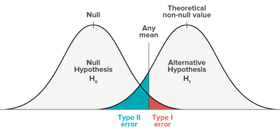
- Type I Error: Pronouncing an innocent person guilty in a criminal trial.
- Type II Error: Declaring a guilty person innocent in a criminal trial.
In hypothesis testing, the objective is to minimize both types of errors, but in practice, we often emphasize one over the other.
- Conservative Approach: Stricter criteria to reduce Type I error.
- Liberal Approach: Looser criteria to reduce Type II error.
The significance level (
It plays a pivotal role in statistical inference, ensuring a balance between Type 1 (false positive) and Type 2 (false negative) errors.
-
Standard Choices:
-
$\alpha = 0.05$ is a common starting point. - Smaller values, like
$\alpha = 0.01$ , are more rigorous.
-
-
Considerations for Application:
- Some domains mandate stringent levels of evidence.
- In early stages of research, a higher
$\alpha$ may be acceptable for hypothesis-generating studies.
A
-
Avoid Data Snooping: Setting
$\alpha$ post-experiment can introduce bias. -
Balance Risks: Adjust
$\alpha$ based on the cost of Type 1 and Type 2 errors. -
Understand Multiplicity Issues: For multiple comparisons,
$\alpha$ should be smaller to maintain overall error rate.
The confidence interval (CI) is a range of values estimated from the sample data that is likely to contain the true parameter of interest, with a certain degree of confidence. It is an essential tool in inferential statistics that helps minimize uncertainty when making inferences about a population from a sample.
-
Quantification of Uncertainty: Confidence intervals provide a measure of uncertainty around an estimate. Instead of relying solely on point estimates, CIs offer a range within which the true population parameter is believed to fall, given the observed sample.
-
Universal Applicability: CIs are used across various statistical methods such as hypothesis testing and parameter estimation, making them a versatile tool in statistical inference.
-
Interpretability: CIs are more intuitive to understand than many p-values. For example, a 95% CI indicates a range of values that, should the study be repeated many times, includes the true population parameter 95% of the time.
The confidence level represents the probability that the CI will contain the true parameter. A common choice is a 95% confidence level, but other levels such as 90% or 99% can be selected based on the specific requirements of the analysis.
The method for calculating a confidence interval varies based on the distribution of the data and the statistic being estimated. For example, for the mean in a normally distributed population:
where:
-
$\bar{X}$ is the sample mean, -
$s$ is the sample standard deviation, -
$n$ is the sample size, and -
$z$ is the z-score associated with the desired confidence level.
For clear interpretation, confidence intervals are often depicted graphically, especially in publications and presentations. This portrayal can communicate the precision of estimates and the existence of statistically significant effects.
- Medical trials often use CIs to assess new drug efficacy.
- In finance, CIs are used to estimate asset returns or default rates.
- CIs are fundamental in political polling to gauge public opinion.
- CIs assist researchers in the evaluation of education and social programs.
-
Sample Size: Larger samples generally lead to narrower CIs, reducing uncertainty.
-
Distribution Assumptions: Many CI calculations assume data follows a specific distribution. For robustness, non-parametric methods can be employed when such assumptions aren't met.
-
Outlier Sensitivity: Extreme values can influence CIs, especially with small samples. Robust estimators or resampling techniques can mitigate this.
-
Multiple Comparisons: When evaluating several groups, the chance of a type I error (false positive) increases. Adjustments like the Bonferroni correction can be made.
-
Two-Tailed vs. One-Tailed: For some applications, decisions focus on only one side of the distribution. In such cases, a one-tailed CI might be more relevant.
-
Practical vs. Statistical Significance: A parameter might be statistically different from a hypothetical value, but that difference may not be practically meaningful. CIs should be interpreted in context.
In statistical hypothesis testing, you distinguish between the null hypothesis
The null hypothesis represents the status quo or the absence of effect. It states that any observed differences in data are due to random variation or chance.
- No Effect or Relationship: Assumption that there is no change or relationship in the population parameters.
- Initial Belief: The starting point, which is upheld unless there is sufficient evidence to reject it.
In an experiment, the null hypothesis often reflects the idea that a new method or treatment has no meaningful effect compared to the existing approach.
The alternative hypothesis is the statement that contradicts the null hypothesis. It asserts that data patterns are a result of a specific effect rather than random variability.
- Presence of an Effect or Relationship: Belief that the population parameters have changed or are related in a specific manner.
- The Hypothesis to Prove: The position that one seeks to establish, usually after having evidence against the null hypothesis.
In the context of an experiment, the alternative hypothesis often represents the idea that a new treatment or method does have a meaningful effect compared to the existing one, or that some relationship or difference in the populations being studied exists.
Bayes' Theorem furnishes an updated probability of an event, taking into account new evidence or information, through the notion of prior and conditional probabilities.
-
Prior Probability
$P(A)$ : The initial belief about an event's probability. -
Likelihood
$P(B|A)$ : The probability of an observed event assuming the cause$A$ . -
Evidence
$P(B)$ : The probability of observing the evidence. -
Posterior Probability
$P(A|B)$ : The updated belief about the event considering the evidence.
Where:
-
$P(A|B)$ : Posterior probability of event A given B -
$P(B|A)$ : Likelihood of B given A -
$P(A)$ : Prior probability of A -
$P(B)$ : Probability of B occurring
-
Medical Diagnosis: Integrate patients' symptoms, tests, and prior probabilities for accurate diagnosis.
-
Spam Filtering: Update the likelihood of certain words matching spam, given prior training data.
-
Data Analysis: For decision making based on incoming data, \textbf{Bayes' Theorem} helps update the probability of different scenarios.
-
A/B Testing: Gauge the effectiveness of two variations by refining the probability of user actions or preferences.
Probability distributions, whether discrete or continuous, play a fundamental role in statistics and machine learning applications, offering insights into the likelihood of various outcomes.
- Discrete: Based on a countable sample space, like the set of all coin toss outcomes: {H, T}.
- Continuous: Defined over an infinite, uncountable sample space, such as all real numbers within a range.
- Discrete: Associated with specific, separate events or values such as the count of heads in a sequence of coin tosses.
- Continuous: Arising from a spectrum of values within a range, typically falling on a number line, for instance, the weight of a person.
- Discrete: For each possible outcome, it provides an exact probability, typically represented by a probability mass function (PMF).
- Continuous: Instead of an exact value, it provides the likelihood of a range of outcomes, typically determined by a probability density function (PDF).
!The PMF represents the probability of discrete random variables taking on specific values. The probabilities for all possible values
!The PDF quantifies the likelihood of continuous random variables falling within a specific interval. It's the derivative of the cumulative distribution function (CDF) with respect to the variable of interest.
-
Expected Value:
- Discrete: Calculated as the sum of each possible value's probability, weighted by the value itself.
- Continuous: Evaluated through the integral of the product of the variable and its PDF over the entire range.
-
Variance:
- Discrete: Obtained by summing the squares of the differences between each value and the expected value, weighted by their probabilities.
- Continuous: Derived from the integral of the squared differences between the variable and its expected value, multiplied by the PDF over the entire range.
- Discrete Distributions: Often used to model count data or categorical outcomes. Examples include the binomial and Poisson.
- Continuous Distributions: Employed in scenarios with measurements or continuous random variables, such as time intervals or real-valued measurements. The normal (Gaussian) and exponential distributions are both continuous distributions.
The Normal Distribution, also known as Gaussian Distribution, is central to many statistical and machine learning techniques. Understanding its key characteristics is essential for data analysis.
-
Bell Shape: The graph resembles a symmetrical bell or a "double-humped" camel. This shape is determined by the specific mean (
$\mu$ ) and standard deviation ($\sigma$ ) of the distribution. - Unimodal: It has a single peak located at its mean.
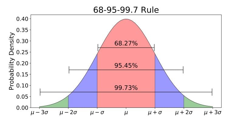
One famous aspect of the Normal Distribution is the empirical rule, which states that:
- Approx. 68% of the data falls within one standard deviation around the mean.
- Approx. 95% of the data falls within two standard deviations around the mean.
- Approx. 99.7% of the data falls within three standard deviations around the mean.
These percentages help to visualize the distribution and are commonly used in building confidence intervals for standard normal distribution.
The distribution is symmetric around the mean, i.e., the area under the curve to the left of the mean is equal to the area to the right.
The tails of the normal distribution approach the
This behavior is often visualized as the distributions tails look parallel to the x-axis in a probability density plot.
While the mean and standard deviation offer insight into the location and spread of the data, the z-score derived from the standard normal distribution can be used to compare observations from different normal populations.
This score provides a measure of how many standard deviations a data point is from the mean.
If
If the mean is zero, the shape of the normal distribution will be such that the tails touch the x-axis at ±1 standard deviation. However, if the mean is non-zero, the point at which the curve touches the x-axis is distinct, determined by the mean and standard deviation.
The normal distribution has been theorized to be optimal due to the central limit theorem. In essence, as the number of observations increases, the distribution of the sample mean tends toward a normal distribution regardless of the shape of the population distribution. Because of this, many statistical tests, such as t-tests and ANOVA, rely on the assumption of normality.
The distribution of normal variates is useful for statistical testing. The extrema (called quantiles) are calculated using Normal(0,1) as a starting point.
For instance, the 95th percentile of a normal distribution corresponds to the value
The Law of Large Numbers (LLN) is a fundamental principle in statistics and probability that describes the convergence of sample statistics to population parameters as the sample size increases.
Put simply, as you gather more data (more observations), the sample mean approaches the true population mean.
This principle underpins many statistical techniques and is crucial for reliable inference.
-
Weak LLN (Averaging Convergence): Establishes that the sample mean converges in probability to the population mean. In simpler terms, the sample mean gets arbitrarily close to the population mean with high probability.
This can be expressed as:
Where:
-
$\bar{X}$ is the sample mean -
$\mu$ is the population mean -
$\varepsilon$ is a small, positive value -
$P$ denotes the probability and the expression says it diminishes to zero as$n$ increases.
- Strong LLN (Absolute Convergence): States that the sample mean converges almost surely to the population mean. This version is stronger than the weak LLN, promising not just convergence in probability, but convergence for almost all individual sample outcomes.
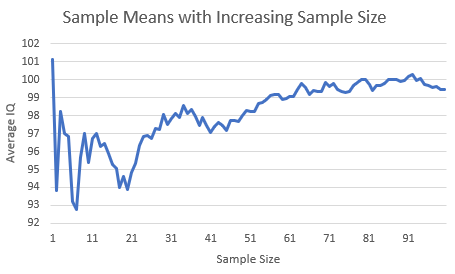
The graph visually represents the strong version of the LLN, showing how the sample mean gets closer to the population mean with increasing sample size.
-
Statistical Inference: Methods such as hypothesis testing and confidence intervals are built on the assumption of the LLN. The convergence of sample statistics like the mean is what allows us to draw conclusions about the population.
-
Decision Making: The LLN provides the logical foundation for making decisions based on data, ensuring that as more information is gathered, our estimates become more reliable.
-
Data Collection Strategy: It emphasizes the significance of sample size, encouraging larger samples for more accurate inferences.
The Binomial distribution essentially models the number of successful outcomes in a fixed number of trials. Its rich theoretical foundation is complemented by real-world utility in diverse fields such as medicine, finance, and quality control.
-
Discreteness: The distribution's output is inherently discrete, ranging from 0 to
$n$ (the number of trials). -
Two-Parameter Design: It characterizes trials via parameters
$n$ and$p$ , representing the number of trials and the probability of success in a single trial, respectively.
-
Quality Control: For example, a manufacturer might use the Binomial distribution to assess the number of defective products in a batch.
-
Finance: In options pricing, the distribution aids in understanding probable stock price movements.
-
Medicine: It is a key tool in clinical trials to decide whether a drug's effectiveness is statistically significant.
-
Genetics: The distribution helps in counting the number of specific genes in a population under given genetic marker conditions.
-
Sports Analytics: It supports predictions about a team's win-loss record based on historical data.
-
Marketing: Marketers can use it to determine the probability of a certain number of successes, like sales, in a given period for a new product or campaign strategy.
-
Machine Learning: It serves as the base for Bernoulli trials used in algorithms such as Naive Bayes.
-
Service Systems: The distribution helps in understanding the probability distribution of the number of customers served within a time interval.
Here is the formula:
where:
-
$P(X = k)$ is the probability of getting$k$ successes in$n$ trials. -
$\binom{n}{k}$ is the binomial coefficient, the number of ways to choose$k$ successes from$n$ trials. -
$p$ is the probability of success in a single trial.
Here is the Python code:
from scipy.stats import binom

# Define parameters
n = 10  # Number of trials
p = 0.3  # Probability of success

# Calculate probabilities
binom_dist = binom(n, p)
binom_dist.pmf(3)  # Probability of 3 successes in 10 trials
Explore all 75 answers here 👉 Devinterview.io - Statistics