
Blogs (English - 中文) | Slides | Poster
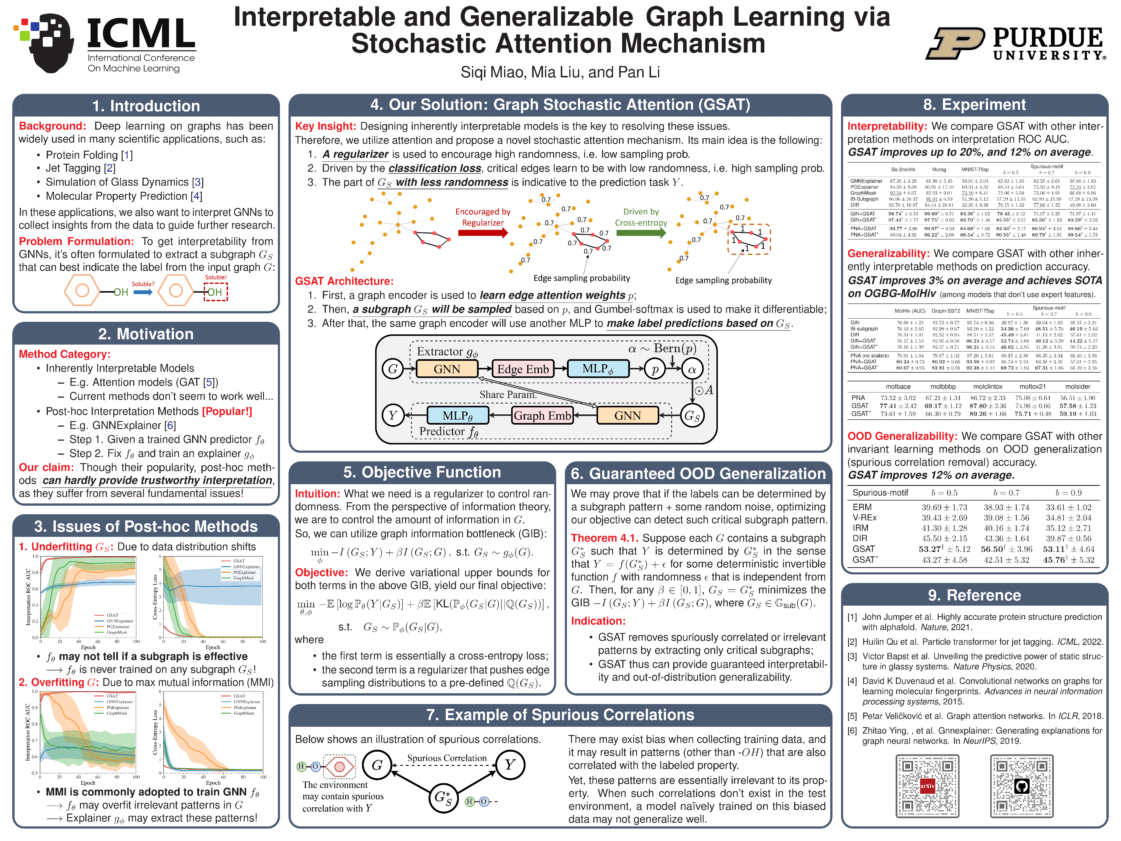
This repository contains the official implementation of GSAT as described in the paper: Interpretable and Generalizable Graph Learning via Stochastic Attention Mechanism (ICML 2022) by Siqi Miao, Mia Liu, and Pan Li.
- Mar. 15, 2023: Check out GSAT on GOOD benchamrk with leaderboard here. GSAT (again) achieves multiple SOTA results on out-of-distribution generalization on the recent benchmark, while being highly interpretable!
- Jan. 21, 2023: Check out our latest paper Learnable Randomness Injection (LRI) with code here, which is recently accepted to ICLR 2023! In LRI, we further generalize the idea of GSAT and propose four datasets with ground-truth interpretation labels from real-world scientific applications (instead of synthetic motif datasets to evaluate interpretability!).
- Nov. 16, 2022: A bug was reported in the code when averaging edge attention weigts for undirected graphs, as pointed out by this issue. We have fixed this bug in the latest version of the code by this PR.
Commonly used attention mechanisms have been shown to be unable to provide reliable interpretation for graph neural networks (GNNs). So, most previous works focus on developing post-hoc interpretation methods for GNNs.
This work shows that post-hoc methods suffer from several fundamental issues, such as underfitting the subgraph
This work addresses those issues by designing an inherently interpretable model. The key idea is to jointly train both the predictor and the explainer with a carefully designed Graph Stochastic Attention (GSAT) mechanism. With certain assumptions, GSAT can provide guaranteed out-of-distribution generalizability and guaranteed inherent interpretability, which makes sure GSAT doesn't suffer from those issues. Fig. 1 shows the architecture of GSAT.

Figure 1. The architecture of GSAT.
The rationale of GSAT is to inject stochasticity when learning attention. For example, Fig 2 shows a task to detect if there exists a five-node-circle in the input graph, so edges with pink end nodes are the critical edges for this task. The main idea of GSAT is the following:
- A regularizer is used to encourage high randomness, i.e. low sampling probability, say
0.7.- In this case, every critical edge may be dropped
30%of the time. - Whenever a critical edge is dropped, it may flip model predictions and incur a huge classification loss.
- In this case, every critical edge may be dropped
- Driven by the classification loss, critical edges learn to be with low randomness, i.e. high sampling probability.
- With high sampling probabilities (e.g.
1.0), the critical edges are more likely to be kept during training.
- With high sampling probabilities (e.g.
- The part with less randomness is the underlying critical data patterns captured by GSAT.
To implement the above mechanism, a proper regularizer is needed. As the goal is to control randomness, from an information-theoretic point of view it's to control the amount of information in Theorem. 4.1. in the paper.

Figure 2. The rationale of GSAT.
We have tested our code on Python 3.9 with PyTorch 1.10.0, PyG 2.0.3 and CUDA 11.3. Please follow the following steps to create a virtual environment and install the required packages.
Clone the repository:
git clone https://github.com/Graph-COM/GSAT.git
cd GSAT
Create a virtual environment:
conda create --name gsat python=3.9 -y
conda activate gsat
Install dependencies:
conda install -y pytorch==1.10.0 torchvision cudatoolkit=11.3 -c pytorch
pip install torch-scatter==2.0.9 torch-sparse==0.6.12 torch-cluster==1.5.9 torch-spline-conv==1.2.1 torch-geometric==2.0.3 -f https://data.pyg.org/whl/torch-1.10.0+cu113.html
pip install -r requirements.txt
In case a lower CUDA version is required, please use the following command to install dependencies:
conda install -y pytorch==1.9.0 torchvision==0.10.0 torchaudio==0.9.0 cudatoolkit=10.2 -c pytorch
pip install torch-scatter==2.0.9 torch-sparse==0.6.12 torch-cluster==1.5.9 torch-spline-conv==1.2.1 torch-geometric==2.0.3 -f https://data.pyg.org/whl/torch-1.9.0+cu102.html
pip install -r requirements.txt
We provide examples with minimal code to run GSAT in ./example/example.ipynb. We have tested the provided examples on Ba-2Motifs (GIN), Mutag (GIN) and OGBG-Molhiv (PNA). Yet, to implement GSAT* one needs to load a pre-trained model first in the provided example. Also try to play with
example.ipynb in Colab.
It should be able to run on other datasets as well, but some hard-coded hyperparameters might need to be changed accordingly, see ./src/configs for all hyperparameter settings. To directly reproduce results for other datasets, please follow the instructions in the following section.
We provide the source code to reproduce the results in our paper. The results of GSAT can be reproduced by running run_gsat.py. To reproduce GSAT*, one needs to first change the configuration file accordingly (from_scratch: false).
To train GSAT or GSAT*:
cd ./src
python run_gsat.py --dataset [dataset_name] --backbone [model_name] --cuda [GPU_id]
dataset_name can be choosen from ba_2motifs, mutag, mnist, Graph-SST2, spmotif_0.5, spmotif_0.7, spmotif_0.9, ogbg_molhiv, ogbg_moltox21, ogbg_molbace, ogbg_molbbbp, ogbg_molclintox, ogbg_molsider.
model_name can be choosen from GIN, PNA.
GPU_id is the id of the GPU to use. To use CPU, please set it to -1.
Standard output provides basic training logs, while more detailed logs and interpretation visualizations can be found on tensorboard:
tensorboard --logdir=./data/[dataset_name]/logs
All settings can be found in ./src/configs.
-
Ba_2Motifs
- Raw data files can be downloaded automatically, provided by PGExplainer and DIG.
-
Spurious-Motif
- Raw data files can be generated automatically, provide by DIR.
-
OGBG-Mol
- Raw data files can be downloaded automatically, provided by OGBG.
-
Mutag
- Raw data files need to be downloaded here, provided by PGExplainer.
- Unzip
Mutagenicity.zipandMutagenicity.pkl.zip. - Put the raw data files in
./data/mutag/raw.
-
Graph-SST2
-
MNIST-75sp
- Raw data files need to be generated following the instruction here.
- Put the generated files in
./data/mnist/raw.
No, GSAT doesn't encourage generating sparse subgraphs. We find r = 0.7 (Eq.(9) in our paper) can generally work well for all datasets in our experiments, which means during training roughly 70% of edges will be kept (kind of still large). This is because GSAT doesn't try to provide interpretability by finding a small/sparse subgraph of the original input graph, which is what previous works normally do and will hurt performance significantly for inhrently interpretable models (as shown in Fig. 7 in the paper). By contrast, GSAT provides interpretability by pushing the critical edges to have relatively lower stochasticity during training.
We recommend to tune r in {0.5, 0.7} and info_loss_coef in {1.0, 0.1, 0.01} based on validation classification performance. And r = 0.7 and info_loss_coef = 1.0 can be a good starting point.
Note that in practice we would decay the value of r gradually during training from 0.9 to the chosen value. Given our empirical observation, the classification performance of GSAT should always be no worse than that yielded by ERM (Empirical Risk Minimization) training, when its hyperparameters are tuned properly.
Recall in Fig. 1, p is the probability of dropping an edge, while α is the sampled result from Bern(p). In our provided implementation, as an empirical choice, α is used to implement Eq.(9) (the Gumbel-softmax trick makes α essentially continuous in practice). We find that when α is used it may provide more regularization and make the model more robust to hyperparameters. Nonetheless, using p can achieve the same performance.
In practice, we don't yield
If you find our paper and repo useful, please cite our paper:
@article{miao2022interpretable,
  title       = {Interpretable and Generalizable Graph Learning via Stochastic Attention Mechanism},
  author      = {Miao, Siqi and Liu, Mia and Li, Pan},
  journal     = {International Conference on Machine Learning},
  year        = {2022}
}