Challenges in High-dimensional Reinforcement Learning with Evolution Strategies

In the following we will provide a quick introduction to working with the code featured in our paper on the "Challenges in High-dimensional Reinforcement Learning with Evolution Strategies".

Although most of the following examples are based on relatively canonical choices of optimization problem and evolution strategy, the steps to follow can have minor differences based on a users pick. Please feel free to check out the documented source code or contact us via the email adresses provided in the paper.

• Start out by cloning the repo.

git clone https://github.com/NiMlr/High-Dim-ES-RL.git
cd High-Dim-ES-RL

• Install the requirements.

# required
pip3 install --upgrade matplotlib numpy
# required only for the RL experiments
pip3 install --upgrade tensorflow keras gym

Contents

Running an evolution strategy on a benchmark

Training an Open-AI Gym controller.

Running an evolution strategy on a benchmark

1. Within a python file import everything we need.

from optimizers import *
from uhoptimizers import *
from benchmarkfunctions import *

import numpy as np
import matplotlib.pyplot as plt
import matplotlib as mpl
mpl.style.use('seaborn')

2. Pick a problem from the following table:

Function(object)	Module	Description
BenignEllipse	benchmarkfunctions.py	A moderately conditioned function.
BenignEllipseNoisyThres	benchmarkfunctions.py	A moderately conditioned function with additive noise above a certain (function value) threshold.
BenignEllipseAddNoise	benchmarkfunctions.py	A stripped down version of the LMMAES implementation. Featuring no CMA or approximation. ES is reasonable to use in extremely high dimension.
BenignEllipseMultNoise	benchmarkfunctions.py	An ES for problems in dimensions >> 100 under uncertainty.
Ellipse	benchmarkfunctions.py	A stripped down version of the UHLMMAES implementation. Featuring no CMA or respective approximation. ES is reasonable to use in extremely high dimensions.
EllipseAddNoise	benchmarkfunctions.py	A badly conditioned function with additive noise of a specified strength applied.
EllipseMultNoise	benchmarkfunctions.py	A badly conditioned function with multiplicative noise of a specified strength applied.
sphere	benchmarkfunctions.py	The standard spherical quadratic function.
SphereAddNoise	benchmarkfunctions.py	The standard spherical quadratic function with additive noise of a specified streght applied.
SphereMultNoise	benchmarkfunctions.py	The standard spherical quadratic function with multiplicative noise of a specified streght applied.

and initialize relevant constants (in case the benchmark function requires these).

# problem dimension
n = 40
# noise amplitude for stochastic function
noiseamp = 1
# get function object
el = EllipseMultNoise(n, noiseamp)

3. Grab some optimizer to test from this table:

Optimizer	Module	Description
LMMAES	optimizers.py	An ES for problems in dimensions >> 100.
MAES	optimizers.py	An ES for problems in dimensions > 100.
ES	optimizers.py	A stripped down version of the LMMAES implementation. Featuring no CMA or approximation. ES is reasonable to use in extremely high dimension.
UHLMMAES	uhoptimizers.py	An ES for problems in dimensions >> 100 under uncertainty.
UHES	uhoptimizers.py	A stripped down version of the UHLMMAES implementation. Featuring no CMA or respective approximation. UHES is reasonable to use in extremely high dimensions under uncertainty.

and initialize it along with these needed input parameters (see respective optimizer docstring for a detailed description).

# logging
performance_log = []

# set initial pop mean
y0    = np.random.randn(n)/n
# initial step size
step_size = 1./6
# initialize optimizer object
esop  = UHLMMAES(y0, step_size, el, function_budget=1e6, threads=8)

4. Now we can start the optimization

# the actual optimization routine
termination = False
while termination is False:
    # optimization step
    evals, solution, termination = esop.step()

    # save some useful values
    performance_log.append( [evals,np.mean(esop.fd)] )
    # print some useful values
    esop.report( 'Appr. fit: %f  Sigma: %f   F-evals: %d\n' %
        (np.mean(esop.fd), esop.sigma, evals) )

and print the result when done.

plt.plot(np.array(performance_log)[:,0], 
 np.log10(np.array(performance_log)[:,1]), linewidth=1)
plt.title('UHLMMAES on ellipse with (multiplicative) noise')
plt.xlabel('function evaluations')
plt.ylabel('$log($population mean fitness$)$')
plt.show()

When sampling the performance of each of the algorithms on the ellipse with multiplicative noise you could end up with a plot like this.

Training an Open-AI Gym controller

1. Within a python file import everything we need.

from optimizers import *
from uhoptimizers import *
from applications.control.gymcontrollers import Controller, Models

import numpy as np
import matplotlib.pyplot as plt
import matplotlib as mpl
mpl.style.use('seaborn')

2. Pick a neural network controller model from the following table:

Model	Module	Description
Models.smallModel	gymcontrollers.py	Primarily used for testing. Neural Net with layers: {input, 10-elu, output-sigmoid}
Models.bipedalModel	gymcontrollers.py	Primarily used in experiments of the bipedal walker. Neural Net with layers: {input, 30-elu, 30-elu, 15-elu, 10-elu, output-sigmoid}
Models.robopongModel	gymcontrollers.py	Primarily used in experiments of robopong game. Neural Net with layers: {input, 30-elu, 30-elu, 15-elu, 10-elu, output-sigmoid}
Models.acrobotModel	gymcontrollers.py	Primarily used in experiments of acrobot game. Neural Net with layers: {input, 30-elu, 30-elu, 10-elu, output-sigmoid}

Alternatively you can use your own model (make sure it is a valid implementation in the following steps and by checking out the gymcontrollers.py module).

3. Initialize the controller. The action space size can not always be determined correctly. Be sure to supply it in these cases.

# gym environment name
env = "Acrobot-v1"
episode_length = 1500

controller = Controller(Models.smallModel, env,
     episode_length, device='/cpu:0', render=False, force_action_space=3)

In order to run controllers on new environments it is mandatory to implement a ActionTransformations method that transforms the action from the neural net output to the respective gym interface. In some cases this method might just return its input. Additionally, a list of thresholds (can be empty, if no interference is needed) can be supplied in the EarlyStop class that feature premature termination of the episode to save runtime. Regarding the implemented environments this must not be kept in mind. For further inquiry: Check out gymcontrollers.py.

4. Run the your favorite Evolution Strategy as introduced in the preceding section.

# logging
performance_log = []

# set initial pop mean
y0    = np.abs(np.random.randn(controller.n))/controller.n
# initial step size
step_size = 0.3
# initialize optimizer object
esop  = UHLMMAES(y0, step_size, controller.fitness, function_budget=1e4, threads=1)

# the actual optimization routine
termination = False
while termination is False:
    # optimization step
    evals, solution, termination = esop.step()
    # save some useful values
    performance_log.append( [evals,np.mean(esop.fd)])
    # print some useful values
    esop.report( 'Appr. fit: %f  Sigma: %f   F-evals: %d\n' %
             (np.mean(esop.fd), esop.sigma, evals) )

Note, that threading is likely not going to work in the current implementation of the gym-controllers (thus set it to 1).

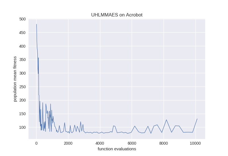
5. Plot and render the result.

controller.render = True
controller.fitness(solution)

plt.plot(np.array(performance_log)[:,0], 
         np.array(performance_log)[:,1], linewidth=1)
plt.title('UHLMMAES on Acrobot')
plt.xlabel('function evaluations')
plt.ylabel('population mean fitness')
plt.show()