DiffEqApproxFun.jl

DiffEqApproxFun.jl is a component package in the DifferentialEquations ecosystem. It holds the components for solving differential equations using spectral methods defined by types from ApproxFun.jl. Users interested in using this functionality should check out DifferentialEquations.jl.

This repository has been deprecated. There are better ways to do this.

Usage Examples

Indirect ApproxFuns

The indirect ApproxFun interface allows one to define an ODEProblem directly from ApproxFun expressions. It will automatically convert this into a spectral ODE problem where the vector is the spectral coefficients. The pro for this method is that it can be used with any ODE solver on the common interface such as Sundials. However, this method uses a constant number of coefficients and truncates the expansions given by ApproxFun to always match this size and so it's a little bit wasteful. But this presents itself as one of the easiest ways to solve a spectral discretization of a PDE.

To define such a problem, we first need to define our inital condition as a Fun type:

using DiffEqApproxFun
S=Fourier()
u0=Fun(θ->cos(cos(θ-0.1))-cos(cos(0-0.1)),S)

Now let's define our ODE which takes in Fun types and spits out new Funs:

c=Fun(cos,S)
ode_prob = ODEProblem((u,p,t)->u''+(c+1)*u',u0,(0.,1.))

To turn this into an indirect ApproxFun problem, we use the ApproxFunProblem wrapper:

prob = ApproxFunProblem(ode_prob)

We can now solve this using any solver:

using OrdinaryDiffEq
sol=solve(prob,Tsit5()) # OrdinaryDiffEq.jl
using Sundials
sol=solve(prob,CVODE_BDF()) # Sundials.jl
using ODEInterfaceDiffEq
sol=solve(prob,radau()) # ODEInterfaceDiffEq.jl

The solution interface works on this output, so to grab the solution at the 5th timepoint we do sol[5] for sol.t[5]. Each solution is a Fun type, which we can evaluate. Thus we can get the value at x=0.2 at time sol.t[5] via sol[5](0.2). The interpolations generate their own Fun types, so the value of x=0.2 at time t=0.5 is calculated via sol(0.5,0.2).

Adding Boundary Conditions

Normally you will want to solve a PDE with non-trivial boundary conditions. If possible you should make your Fun discretization match the BCs. For example, this is done automatically when the BCs are periodic and the discretization is periodic. But this isn't always possible, in which case you will need to define a bc function which projects the solution at each step to satisfy the boundary conditions. For example, we can have Dirichlet conditions s.t. the solution must be zero at the endpoints of our interval in the problem above via:

function bc(t,u)
  C=eye(S)[3:end,:]
  tmp = [Evaluation(0);
         Evaluation(2π);
         C]\[0.;0.;u]
end

Then we can generate a callback via BoundaryCallback and have the solver utilize this callback. This requires a common interface solver which is compatible with the callback interface.

boundary_projection = BoundaryCallback(bc)
sol=solve(prob,Tsit5(),callback=boundary_projection)

The resulting solution satisfies the boundary conditions.

Plotting

Note that sol(0.5) returns the interpolated Fun type at time t=0.5, and Fun types have their own plotting recipes. Thus you can plot the solution at snippets of time directly like plot(sol(0.5)). Example:

plot(sol[1],labels="t=0.0") 
plot!(sol(0.5),labels="t=0.5")
plot!(sol[end],labels="t=1.0")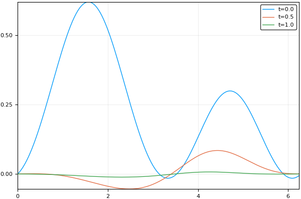

Direct ApproxFuns

The direct ApproxFun interface is simply using a Fun as an initial condition and a function on Fun types as the function in a standard ODEProblem. The *DiffEq solvers like OrdinaryDiffEq.jl will directly handle this as an adaptive-space spectral discretization of the PDE. However, care has to be taken since this can cause the number of coefficients to grow rapidly. One may need to use an L-stable integrator and change the linear solver which is used. This is still in development.