fourier_series_fitimplements the Fourier series fitting of periodic scalar functions using a series of trigonometric functions.
fit.best_fit()implements the main fitting function. Given a series of 2D, scalar data points(xs, Fs)and a penalty functionp,fit.best_fit(xs, Fs, penalty_function=p)returns a list of terms as well as a measure of the goodness of fit (weighted and unweight root mean square deviation). The list of terms can be used to crate an interpolation function usingfourier_series_fct(list_of_terms)used to evaluate the fitting function at any point.
Cf example_trigonometric.py:
from numpy import linspace, pi, cos, random
from fit import best_fit, fourier_series_fct, LINEAR_PENALTY_FUNCTION
# Get 40 points linearly distributed between -pi and pi
xs = linspace(-pi, pi, 40)
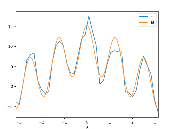
# F(x) = 5 + 4.cos(x) + 6.cos(5x), with some Gaussian noise
Fs = 5.0 + 4. * cos(xs) + 6. * cos (5 * xs) + 1.5 * random.normal(0, 1.0, len(xs))
# Fit with a linear penalty function P: terms -> 1.0 * len(terms)
fit_terms, weighted_rmsd, unweighted_rmsd = best_fit(xs, Fs, penalty_function=LINEAR_PENALTY_FUNCTION)
interpolated_fct = fourier_series_fct(fit_terms)
# Evaluate the fitting function on 200 equally distributed points between -pi and pi
fine_xs = linspace(-pi, pi, 200)
interpolated_Fs = [interpolated_fct(x) for x in fine_xs]
print('Fit terms:', fit_terms)
# Plot F and its fit
import pylab as p
p.plot(xs, Fs, label='F')
p.plot(fine_xs, interpolated_Fs, label='fit')
p.xlabel('$\phi$')
p.xlim([-pi, pi])
p.legend()
p.show()
# Re-run with debugging on to see the effect of the penalty function
from sys import stderr
fit_terms, weighted_rmsd, unweighted_rmsd = best_fit(xs, Fs, penalty_function=LINEAR_PENALTY_FUNCTION, debug=stderr)
Cf example_trigonometric.py:
from numpy import linspace, cos, pi
from fit import get_fourier_terms, fourier_series_fct
from rmsd import vector_rmsd
import pylab as p
xs_in_rad = linspace(-pi, pi, 500)
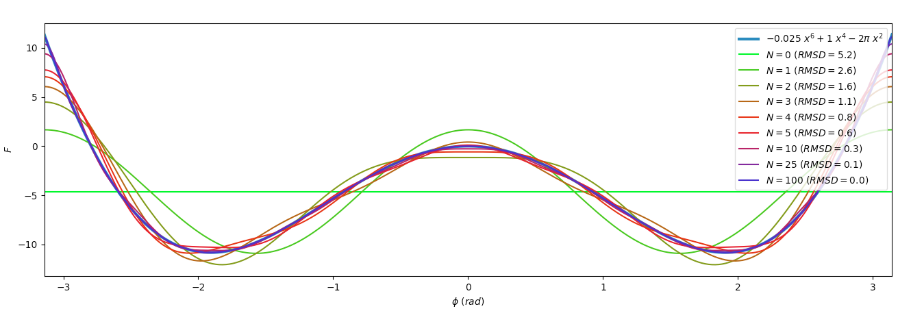
FUNCTION_LATEX_FORM, FUNCTION = ('$-0.025 \ x^6 + 1 \ x^4 - 2 \pi \ x^2$', lambda xs: - 0.025 * xs ** 6 + xs ** 4 - 2 * pi * xs ** 2)
Es = FUNCTION(xs_in_rad)
all_terms = get_fourier_terms(xs_in_rad, Es, range(1, 100))
sorted_terms = sorted(
all_terms,
key=lambda term: (term.n != 0, -abs(term.k_n)),
)
figure, axis = p.subplots()
axis.plot(xs_in_rad, Es, label=FUNCTION_LATEX_FORM, linewidth=3.0)
cmap = p.get_cmap('brg')
Ns = [0, 1, 2, 3, 4, 5, 10, 25, 100]
for (i, N) in enumerate(Ns):
print(N, sorted_terms[:N + 1])
fit_fct = fourier_series_fct(sorted_terms[:N + 1])
axis.plot(
xs_in_rad,
fit_fct(xs_in_rad),
label='$N={0:<3d}\ (RMSD={1:.1f})$'.format(N, vector_rmsd(Es, fit_fct(xs_in_rad))),
marker='',
linestyle='-',
color=cmap(1.0 - (i / (len(Ns) * 1.))),
)
axis.set_xlabel('$\phi\ (rad)$')
axis.set_ylabel('$F$')
axis.set_xlim((-pi, pi))
NCOLS = 1
axis.legend(loc='upper right', scatterpoints=1)
p.show()