
Illustration by vectorjuice - www.freepik.com
Introduction
Methodology
Requirements
Execution Guide
Data Acquisition
Data Preparation
Raw Data Description
Data Exploration
Modeling
Summary
Front-end
Conclusions
References
About Me
While working in a company that serves goods to thousands of customers in several countries, I wanted to create a tool that would be useful to the sales managers in those countries by quickly showcasing what customers to contact next, in order to grow sales and customer retention. That is how I came to know about RFM analysis.
RFM is a method used for analyzing customer value. It is commonly used in database marketing and direct marketing and has received particular attention in retail and professional services industries.
This project focuses on doing RFM analysis on company sales and creating a data visualization dashboard showcasing customer segmentation that I can share with colleagues in the countries.

Using a dataset that contains sales orders in a period of time, we will use Python to obtain the frequency, recency and monetary values in the last 365 days per customer. Later with those values we will give R, F, and M scores to each customer, that will allow us to cluster them in different segments.
We'll use the Google Colaboratory Jupyter notebook environment (free), with Python 3.7 or higher, and Microsoft Power BI Desktop application (free download, Windows only).
- numpy
- pandas
- math
- datetime
- dataprep
- matplotlib
For replicating the project, please execute the following steps in order:
-
Jupyter notebook. Running this notebook the data will be explored, prepared, and the RFM segmentation will be performed. The output will be a CSV file.
-
Power BI file. This is a file that processes the CSV file obtained in the previous step and presents it as a dashboard so it can be leveraged for business actions in the countries.
Data has been obtained from real sales orders in 18 countries in a period of around 2 years. Some features (country names, customer id and revenue), have been altered in order to preserve privacy. Number of orders, units and dates have not been modified. It is acquired as a CSV file.
We import the CSV and we put it into a dataframe with pandas. We know from domain knowledge that every row of the dataset is a different order.
df1.head()
| country | id | week.year | revenue | units | |
|---|---|---|---|---|---|
| 0 | KR | 702234 | 03.2019 | 808.08 | 1 |
| 1 | KR | 702234 | 06.2019 | 1606.80 | 2 |
| 2 | KR | 3618438 | 08.2019 | 803.40 | 1 |
| 3 | KR | 3618438 | 09.2019 | 803.40 | 1 |
| 4 | KR | 3618438 | 09.2019 | 803.40 | 1 |
Also, we notice that the date is expressed as week of the year, so for better analysis we convert it to year-month-day format with the datetime package. Also we rename 'revenue' to 'monetary' per convention in the RFM analysis.
df2.head()
| country | id | monetary | units | date | |
|---|---|---|---|---|---|
| 0 | KR | 702234 | 808.08 | 1 | 2019-01-21 |
| 1 | KR | 702234 | 1606.80 | 2 | 2019-02-11 |
| 2 | KR | 3618438 | 803.40 | 1 | 2019-02-25 |
| 3 | KR | 3618438 | 803.40 | 1 | 2019-03-04 |
| 4 | KR | 3618438 | 803.40 | 1 | 2019-03-04 |
df2.info()
class 'pandas.core.frame.DataFrame';
RangeIndex: 235574 entries, 0 to 235573
Data columns (total 5 columns):
 #   Column    Non-Null Count   Dtype
---  ------    --------------   -----
 0   country   235574 non-null  object
 1   id        235574 non-null  int64
 2   monetary  235574 non-null  float64
 3   units     235574 non-null  int64
 4   date      235574 non-null  datetime64[ns]
dtypes: datetime64[ns](1), float64(1), int64(2), object(1)
memory usage: 9.0+ MB
df2.describe()
| id | monetary | units | |
|---|---|---|---|
| count | 2.355740e+05 | 2.355740e+05 | 235574.000000 |
| mean | 3.193118e+06 | 2.840211e+03 | 8.599642 |
| std | 7.371744e+06 | 2.247532e+04 | 602.939290 |
| min | 6.000180e+05 | -1.061539e+05 | -150000.000000 |
| 25% | 2.214396e+06 | 3.994800e+02 | 1.000000 |
| 50% | 3.140856e+06 | 1.150320e+03 | 1.000000 |
| 75% | 3.892650e+06 | 2.216160e+03 | 2.000000 |
| max | 2.419308e+08 | 2.415857e+06 | 150000.000000 |
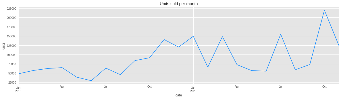
We see we have 235,574 transactions and 5 columns in the period of time included in the dataset. The biggest transaction was 150,000 units. But it seems there was a return of that amount as well, -150,000 units. The most expensive purchase was 2.41 Millions.
Let's view the period of time included in the dataset:
df2['date'].min()
Timestamp('2019-01-07 00:00:00')
df2['date'].max()
Timestamp('2020-11-30 00:00:00')
Let's explore in how many different countries we have sales in that period:
df2['country'].unique()
array(['KR', 'PK', 'MM', 'VN', 'IN', 'SA', 'PH', 'AF', 'CN', 'BD', 'ID',
       'TH', 'IQ', 'MY', 'JP', 'IR', 'TR', 'UZ'], dtype=object)
With the dataprep.clean package we can get the full country names:
clean_country(df2, "country")['country_clean'].unique()
array(['South Korea', 'Pakistan', 'Myanmar', 'Vietnam', 'India',
       'Saudi Arabia', 'Philippines', 'Afghanistan', 'China',
       'Bangladesh', 'Indonesia', 'Thailand', 'Iraq', 'Malaysia', 'Japan',
       'Iran', 'Turkey', 'Uzbekistan'], dtype=object)
Total number of customers in all countries:
df2['id'].nunique()
21837
For greater visibility in the plots we convert the dates to monthly periods:
df2c = df2b.to_period("M")
df2c.head()
| country | id | monetary | units | |
|---|---|---|---|---|
| date | ||||
| 2019-01 | KR | 702234 | 808.08 | 1 |
| 2019-02 | KR | 702234 | 1606.80 | 2 |
| 2019-02 | KR | 3618438 | 803.40 | 1 |
| 2019-03 | KR | 3618438 | 803.40 | 1 |
| 2019-03 | KR | 3618438 | 803.40 | 1 |
We aggregate the units and revenue of the same period.
Units chart:
df2c['units'].groupby('date').agg(sum).plot(figsize=(20,5));
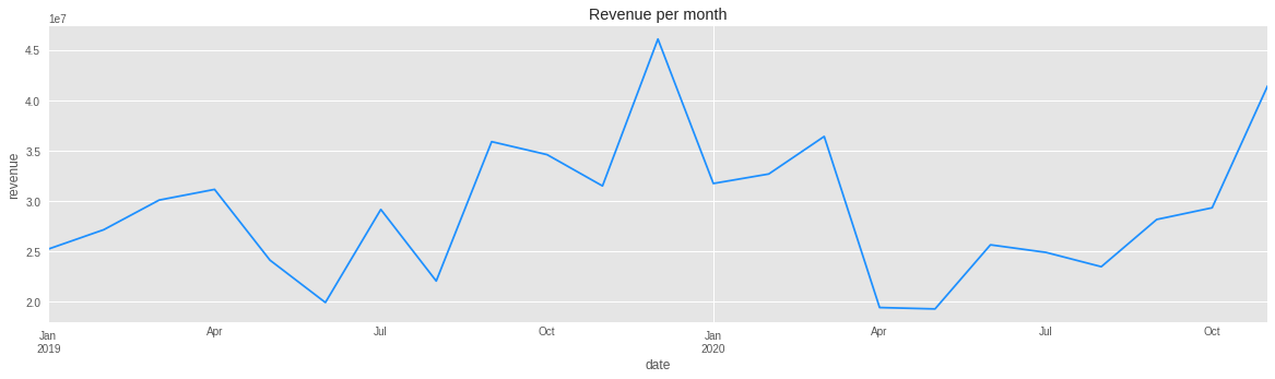
Revenue chart:
df2c['monetary'].groupby('date').agg(sum).plot(figsize=(20,5));
We will transform the data to assign each customer some scores depending on the purchases they did. Prior to that, we will create some new features 'recency', 'frequency', as long as the previoulsy created 'monetary' feature.
Recency will be the minimum of 'days_since_last_purchase' for each customer.
Frequency will be the total number of orders in the period for each customer.
Monetary, will be the total value of the purchases in the period for each customer.
We will focus on sales from last 365 days since the most recent date.
TIP: There are customers with the same 'id' in several countries. This causes errors in the monetary values. We will solve this by creating a new feature: a unique 'id+' identifier that combines country code and customer id.
df3['id+'] = df3['country'].map(str) + df3['id'].map(str)
df3.head()
| country | id | monetary | units | date | id+ | days_since_purchase | |
|---|---|---|---|---|---|---|---|
| 0 | KR | 4375152 | 773.58 | 1 | 2019-12-16 | KR4375152 | 351 |
| 1 | KR | 705462 | 337.26 | 1 | 2019-12-09 | KR705462 | 358 |
| 2 | KR | 705462 | 337.26 | 1 | 2019-12-23 | KR705462 | 344 |
| 3 | KR | 705462 | 421.56 | 2 | 2019-12-16 | KR705462 | 351 |
| 4 | KR | 706854 | 391.50 | 1 | 2019-12-09 | KR706854 | 358 |
The result will be a dataframe that contains two new columns: 'recency' and 'frequency'.
rfm.head()
| id | id+ | country | recency | frequency | monetary | |
|---|---|---|---|---|---|---|
| 0 | 600018 | CN600018 | CN | 29 | 7 | 21402.78 |
| 1 | 600060 | CN600060 | CN | 155 | 1 | 1201.14 |
| 2 | 600462 | CN600462 | CN | 211 | 2 | 2033.64 |
| 3 | 600888 | CN600888 | CN | 8 | 3 | 2335.80 |
| 4 | 601014 | CN601014 | CN | 225 | 1 | 230.52 |
No we'll assign a rate between 1 and 5 depending on recency, monetary and frequency parameters. We'll use the quintiles method, dividing every feature on groups that contain 20 % of the samples.
Higher values are better for frequency and monetary, while lower values are better for recency. Those will be the asssigned R, F and M scores to each customer.
Then we concatenate R, F and M values to obtain a combined RFM score per customer.
rfm.head()
| id | country | recency | frequency | monetary | r | f | m | rfm_score | |
|---|---|---|---|---|---|---|---|---|---|
| 0 | 600018 | CN | 29 | 7 | 21402.78 | 4 | 4 | 5 | 445 |
| 1 | 600060 | CN | 155 | 1 | 1201.14 | 2 | 1 | 2 | 212 |
| 2 | 600462 | CN | 211 | 2 | 2033.64 | 2 | 2 | 2 | 222 |
| 3 | 600888 | CN | 8 | 3 | 2335.80 | 5 | 3 | 3 | 533 |
| 4 | 601014 | CN | 225 | 1 | 230.52 | 2 | 1 | 1 | 211 |
With this rfm scores we would have 125 segments of customers, which is too much for any practical analysis. To get a more simple segmentation, we choose to create a new feature 'fm' that is the rounded down mean of 'f' and 'm' scores.
def truncate(x): return math.trunc(x)
rfm['fm'] = ((rfm['f'] + rfm['m'])/2).apply(lambda x: truncate(x))
| id | country | recency | frequency | monetary | r | f | m | rfm_score | fm | |
|---|---|---|---|---|---|---|---|---|---|---|
| 0 | 600018 | CN | 29 | 7 | 21402.78 | 4 | 4 | 5 | 445 | 4 |
| 1 | 600060 | CN | 155 | 1 | 1201.14 | 2 | 1 | 2 | 212 | 1 |
| 2 | 600462 | CN | 211 | 2 | 2033.64 | 2 | 2 | 2 | 222 | 2 |
| 3 | 600888 | CN | 8 | 3 | 2335.80 | 5 | 3 | 3 | 533 | 3 |
| 4 | 601014 | CN | 225 | 1 | 230.52 | 2 | 1 | 1 | 211 | 1 |
Then we create a segment map of only 11 segments based on only two scores, 'r' and 'fm'. We assign to each customer a different segment.
| id | country | recency | frequency | monetary | r | fm | segment | |
|---|---|---|---|---|---|---|---|---|
| 0 | 600018 | CN | 29 | 7 | 21402.78 | 4 | 4 | loyal customers |
| 1 | 600060 | CN | 155 | 1 | 1201.14 | 2 | 1 | lost |
| 2 | 600462 | CN | 211 | 2 | 2033.64 | 2 | 2 | hibernating |
| 3 | 600888 | CN | 8 | 3 | 2335.80 | 5 | 3 | potential loyalists |
| 4 | 601014 | CN | 225 | 1 | 230.52 | 2 | 1 | lost |
After aggregating sales, frequency and recency values for each customer, and assigning 'r' and 'fm' scores depending on those values, we have given each customer a different segment label. Let's have a look on what those segments mean.
- Champions Bought recently, buy often and spend the most
- Loyal Customers Buy on a regular basis. Responsive to promotions.
- Potential Loyalists Recent customers with average frequency.
- Recent Customers Bought most recently, but not often.
- Promising Recent shoppers, but haven’t spent much.
- Customers Needing Attention Above average recency, frequency and monetary values. May not have bought very recently though.
- About To Sleep Below average recency and frequency. Will lose them if not reactivated.
- At Risk Purchased often but a long time ago. Need to bring them back!
- Can’t Lose Them Used to purchase frequently but haven’t returned for a long time.
- Hibernating Last purchase was long back and low number of orders.
- Lost Purchased long time ago and never came back.
We can display some customer segments in the dataframe.
Can't lose
rfm[rfm['segment']=="can't lose"].sort_values(by='monetary', ascending=False).head()
| id | country | recency | frequency | monetary | r | fm | segment | |
|---|---|---|---|---|---|---|---|---|
| 13028 | 4096386 | JP | 260 | 105 | 220267.86 | 1 | 5 | can't lose |
| 3502 | 2443284 | IN | 246 | 10 | 102208.02 | 1 | 5 | can't lose |
| 14174 | 4262646 | IN | 316 | 10 | 91909.44 | 1 | 5 | can't lose |
| 2435 | 1803672 | IN | 267 | 12 | 70506.96 | 1 | 5 | can't lose |
| 13254 | 4132968 | VN | 253 | 26 | 42535.14 | 1 | 5 | can't lose |
Loyal customers
rfm[rfm['segment']=='loyal customers'].sort_values(by='monetary', ascending=False).head()
| id | country | recency | frequency | monetary | r | fm | segment | |
|---|---|---|---|---|---|---|---|---|
| 15420 | 4422780 | TR | 92 | 13 | 2315341.14 | 3 | 5 | loyal customers |
| 2882 | 2030526 | JP | 22 | 50 | 1519339.86 | 4 | 5 | loyal customers |
| 3220 | 2182446 | JP | 29 | 18 | 1492057.68 | 4 | 5 | loyal customers |
| 12660 | 4041366 | PK | 50 | 9 | 736626.96 | 4 | 4 | loyal customers |
| 5612 | 2853774 | VN | 8 | 6 | 712230.00 | 5 | 4 | loyal customers |
Champions
rfm[rfm['segment']=='champions'].sort_values(by='monetary', ascending=False).head()
| id | country | recency | frequency | monetary | r | fm | segment | |
|---|---|---|---|---|---|---|---|---|
| 173 | 638544 | CN | 1 | 217 | 21482332.56 | 5 | 5 | champions |
| 15436 | 4424580 | CN | 1 | 104 | 16912322.46 | 5 | 5 | champions |
| 14754 | 4341960 | TR | 1 | 200 | 16550997.90 | 5 | 5 | champions |
| 11942 | 3929094 | ID | 1 | 470 | 8748884.64 | 5 | 5 | champions |
| 9626 | 3520734 | JP | 1 | 198 | 6207519.96 | 5 | 5 | champions |
Customers with monetary over the average that need attention
rfm[(rfm['monetary']>rfm['monetary'].mean()) & (rfm['segment']=='need attention')].sort_values(by='monetary', ascending=False).head()
| id | country | recency | frequency | monetary | r | fm | segment | |
|---|---|---|---|---|---|---|---|---|
| 8245 | 3242664 | TR | 64 | 1 | 73823.58 | 3 | 3 | need attention |
| 13065 | 4107798 | JP | 120 | 2 | 67257.48 | 3 | 3 | need attention |
| 9847 | 3561900 | ID | 120 | 1 | 59700.00 | 3 | 3 | need attention |
| 6626 | 2921070 | ID | 71 | 2 | 34730.22 | 3 | 3 | need attention |
| 10009 | 3587772 | CN | 92 | 1 | 29961.00 | 3 | 3 | need attention |
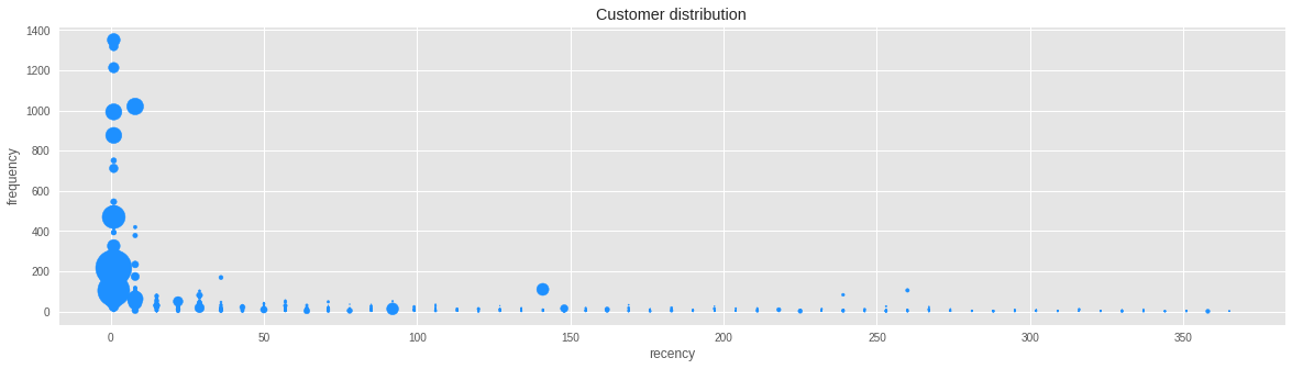
Let's do a scatter plot to explore the distribution of customers, with 'recency' on the x-axis and 'frequency' in the y-axis. Using the 'monetary' values as size of the points, we see that the majority of customers who spend the most also purchase more recently and more frequently.
Finally we export the dataframe to a CSV file for later processing it in Power BI.
rfm.to_csv('rfm_asia.csv', encoding='utf-8', index=False, float_format='%.2f')
The front-end of this project consists in a Power BI dashboard that processes the CSV resulting from executing the previous Python code, and visualizes the results in a pleasing dashboard. That dashboard then can be shared with multiple colleagues in the different countries of the company. You can access that file here for exploring it.


We observe that a lot of our customers (32 %) are lost or hibernating (they have a few orders from long ago). However, 28 % of our customers are either champions or loyal customers, meaning they spend the most and frequently. A segment to take care is can't lose, second segment with highest revenue, comprised of customers who used to spend a lot but have not returned in a while.
We can share the dashboard with our country sales managers so they can be guided to the customer id's on the different segments and take specific actions on them. Let's view an example: my Chinese colleague needs to be guided on what customers to contact next to improve customer retention or to increase sales. They would just need to open this dashboard, click on country (top right) and then on customer segment need attention or at risk, to have a specific list of customers, ordered by revenue spent in the last 365 days. (An unedited dataset would also include customer names and contact details, which in this case have been omitted for privacy reasons).


A reference guide to the 11 segments and suggested actions per segment is included in the last tab of the dashboard.

Customer segmentation with the RFM methodology in sales is an effective way to help employees to focus their efforts by targeting customers on a priority basis and taking different actions on them. This kind of project flexible as the number of segments can be adapted to the business needs, and the period of time in the analysis can be extended or reduced as well. The use of Power BI to share the dashboard to colleagues in an enterprise environment as a web app is very convenient for companies already working in the Microsoft ecosystem.
Guillaume Martin - RFM Segmentation with Python
Google Cloud - Predicting Customer Lifetime Value with AI Platform