The PyPore package is based off of a few core data analysis packages in order to provide a consistent and easy framework for handling nanopore data in the UCSC nanopore lab. The packages it requires are:
- numpy
- scipy
- matplotlib
- sklearn
Packages which are not required, but can be used, are:
- mySQLdb
- cython
- PyQt4
Let's get started!
There are several core datatypes implemented in order to speed up analysis. These are currently File, Event, and Segment. Each of these is a way to store a full, or parts of, a .abf file and perform common tasks.
- Attributes: duration, mean, std, min, max, n (# events), second, current, sample, events, event_parser, filename
- Instance Methods: parse( parser ), delete(), to_meta(), to_json( filename ), to_dict(), to_database( database, host, user, password ), plot( color_events )
- Class Methods: from_json( filename ), from_database( ... )
Nanopore data files consist primarily of current levels corresponding to ions passing freely through the nanopore ("open channel"), and a blockages as something passes through the pore, such as a DNA strand ("events"). Data from nanopore experiments are stored in Axon Binary Files (extension .abf), as a sequence 32 bit floats, and supporting information about the hardware. They can be opened and loaded with the following:
from PyPore.DataTypes import *
file = File( "My_File.abf" )
The File class contains many methods to simplify the analysis of these files. The simplest analysis to do is to pull the events, or blockages of current, from the file, while ignoring open channel. Let's say that we are looking for any blockage of current which causes the current to dip from an open channel of ~120 pA. To be conservative, we set the threshold the current has to dip before being significant to 110 pA. This can be done simply with the file's parse method, which requires a parser class which will perform the parsing. The simplest event detector is the lambda_event_parser, which has a keyword threshold, indicating the raw current that serves as the threshold.
from PyPore.DataTypes import *
file = File( "My_File.abf" )
file.parse( parser=lambda_event_parser( threshold=50 ) )
The events are now stored as Event objects in file.events. The only other important file methods involve loading and saving them to a cache, which we'll cover later. Files also have the properties mean, std, and n (number of events). If we wanted to look at what it thought were events, we could use the plot method. By default, this method will plot detected events in a different color.
from PyPore.DataTypes import *
file = File( "My_File.abf" )
file.parse( parser=lambda_event_parser( threshold=50 ) )
file.plot()

Given that a file is huge, only every 100th point is used in the black regions, and every 5th point is used in events. This may lead to some problems, such as there are two regions which seem like they should be called events, but are colored black and not cyan. This is because in reality, there are spikes below 0 in each of these segments, and the parsing method filtered out any events which went below 0 pA at any point. However, the downsampling removed this spike (because it was less than 100 points long).
- Attributes: duration, start, end, mean, std, min, max, n, current, sample, segments, state_parser, filtered, filter_order, filter_cutoff
- Instance Methods: filter( order, cutoff ), parse( parser ), delete(), apply_hmm( hmm ), plot( [hmm, kwargs), to_meta(), to_dict(), to_json()
- Class Methods: from_json( filename ), from_database( ... ), from_segments( segments )
Events are segments of current which correspond to something passing through the nanopore. We hope that it is something which we are interested in, such as DNA or protein. An event is usually made up of a sequence of discrete segments of current, which should correspond to reading some region of whatever is passing through. In the best case, each discrete segment in an event corresponds to a single nucleotide of DNA, or a single amino acid of a protein passing through.
Events are often noisy, and transitions between them are quick, making filtering a good option for trying to see the underlying signal. Currently only bessel filters are supported for filtering tasks, as they've been shown to perform very well.
Let's continue with our example, and imagine that now we want to filter each event, and look at it! The filter method has two parameters, order and cutoff, defaulting to order=1 and cutoff=2000. (Note that we now import pyplot as well.)
from PyPore.DataTypes import *
from matplotlib import pyplot as plt

file = File( "My_File.abf" )
file.parse( parser=lambda_event_parser( threshold=50 ) )

for event in file.events:
    event.filter( order=1, cutoff=2000 )
    event.plot()
    plt.show()

The first event plotted in this loop is shown.
Currently, lambda_event_parser and MemoryParse are the most used File parsers. MemoryParse takes in two lists, one of starts of events, and one of ends of events, and will cut a file into it's respective events. This is useful if you've done an analysis before and remember where the split points are.
The plot command will draw the event on whatever canvas you have, allowing you to make subplots with the events or add them into GUIs (such as Abada!), with the downside being that you need to use plt.show() after calling the plot command. The plot command wraps the pyplot.plot command, allowing you pass in any argument that could be used by pyplot.plot, for example:
event.plot( alpha=0.5, marker='o' )

This plot doesn't look terrible good, and takes longer to plot, but it is possible to do!
Subplot handling is extremely easy. All of the plotting commands plot to whichever canvas is currently open, allowing for you to do something like this:
from PyPore.DataTypes import *
from matplotlib import pyplot as plt

file = File( "My_File.abf" )
file.parse( parser=lambda_event_parser( threshold=50 ) )

for event in file.events:
    plt.subplot(211)
    event.plot()
    plt.subplot(212)
    event.filter()
    event.plot()
    plt.show()
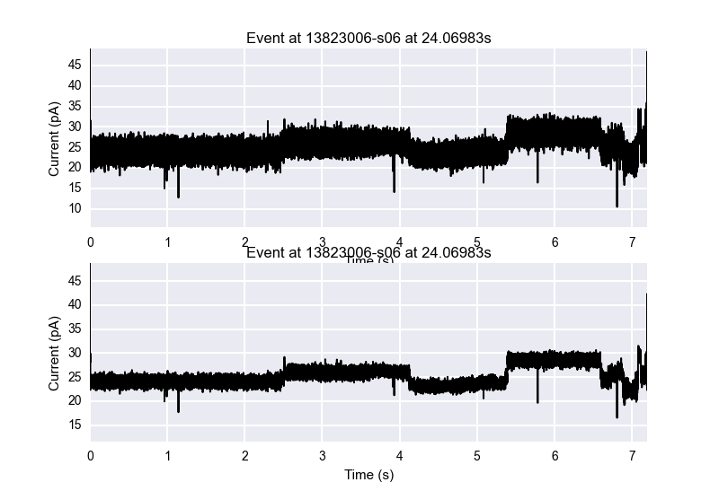
This plot shows how easy it is to show a comparison between an event which is not filtered versus one which is filtered.
The next step is usually to try to segment this event into it's discrete states. There are several segmenters which have been written to do this, of which currently *StatSplit is the best, written by Dr. Kevin Karplus and based on a recursive maximum likelihood algorithm. This algorithm was sped up by rewritting it in Cython, leading to *SpeedyStatSplit, which is a python wrapper for the cython code. Segmenting an event is the same process as detecting events in a file, by using the parse method on an event and passing in a parser.
Let's say that now we want to segment an event and view it. Using the same plot command for the event, we can specify to color by 'cycle', which colors the segments in a four-color cycle for easy viewing. SpeedyStatSplit takes in several parameters, of which *min_gain_per_sample is the most important, and 0.50 to 1.50 usually provide an adequate level to parse at, with higher numbers leading to less segments.
from PyPore.DataTypes import *
from matplotlib import pyplot as plt

file = File( "My_File.abf" )
file.parse( parser=lambda_event_parser( threshold=50 ) )

for event in file.events:
    event.filter( order=1, cutoff=2000 )
    event.parse( parser=SpeedyStatSplit( min_gain_per_sample=0.50 ) )
    event.plot( color='cycle' )
    plt.show()

The color cycle goes blue-red-green-cyan.
The most reliable segmenter currently is SpeedyStatSplit. For more documentation on the parsers, see the parsers segment of this documentation. Both Files and Events inherit from the Segment class, described below. This means that any of the parsers will work on either files or events.
The last core functionality is the ability to apply an hidden markov model (HMM) to an event, and see which segments correspond to which hidden states. HMM functionality is made possible through the use of the yahmm class, which has a Model class and a viterbi method, which is called to find the best path through the HMM. A good example of one of these HMMs is tRNAbasic or tRNAbasic2, which were both made for this purpose. Lets say we want to compare the two HMMs to see which one we agree with more.
from PyPore.DataTypes import *
from PyPore.hmm import tRNAbasic
from matplotlib import pyplot as plt

file = File( "My_File.abf" )
file.parse( lambda_event_parser( threshold=50 ) )

for i, event in enumerate( file.events ):
	event.filter()
	event.parse( SpeedyStatSplit( min_gain_per_sample=.2 ) )
	plt.subplot( 411 )
	event.plot( color='cycle' )

	plt.subplot( 412 )
	event.plot( color='hmm', hmm=tRNAbasic() )

	plt.subplot( 413 )
	event.plot( color='hmm', hmm=tRNAbasic2() )

	plt.subplot( 414 )
	plt.imshow( [ np.arange(11) ], interpolation='nearest', cmap="Set1" )
	plt.grid( False )

	means = [ 33, 29.1, 24.01, 26.04, 24.4, 29.17, 27.1, 25.7, 22.77, 30.06, 24.9 ]
	for i, mean in enumerate( means ):
		plt.text( i-0.2, 0.1, str(mean), fontsize=16 )

	plt.show()
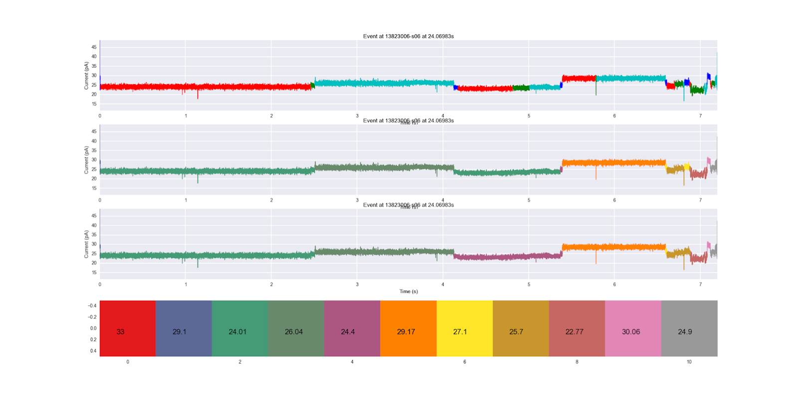
You'll notice that the title of an image and the xlabel of the image above it will always conflict. This is unfortunate, but an acceptable consequence in my opinion. If you're making more professional grade images, you may need to go in and manually fix this conflict. We see the original segmentation on the top, the first HMM applied next, and the second HMM on the bottom. The color coding of each HMM hidden state (sequentially) along with the mean ionic current of their emission distribution are shown at the very bottom. We see that the bottom HMM seems to progress more sequentially, progressing to the purple state instead of regressing back to the blue-green state in the middle of the trace. It also does not go backwards to the yellow state once it's in the gold state later on in the trace. It seems like a more robust HMM, and this way of comparing them is super easy to do.
Event objects also have the properties start, end, duration, mean, std, and n (number of segments after segmentation has been performed).
- Attributes: duration, start, end, mean, std, min, max, current
- Instance Methods: to_json( filename ), to_dict(), to_meta(), delete()
- Class Methods: from_json( filename )
A segment stores the series of floats in a given range of ionic current. This abstract notion allows for both Event and File to inherit from it, as both a file and an event are a range of floats. The context in which you will most likely interact with a Segment is in representing a discrete step of the biopolymer through the pore, with points usually coming from the same distribution.
Segments are short sequences of current samples, usually which appear to be from the same distribution. They are the core place where data are stored, as usually an event is analyzed by the metadata stored in each state. Segments have the attributes current, which stores the raw current samples, in addition to mean, std, duration, start, end, min, and max.
If storing the raw sequence of current samples is too memory intensive, there are two ways to get rid of lists of floats representing the current, which take up the vast majority of the memory ( >~99% ).
- Initialize a MetaSegment object, instead of a Segment one, and feed in whatever statistics you'd like to save. This will prevent the current from ever being saved to a second object. For this example, lets assume you have a list of starts and ends of segments in an event, such as loading them from a cache.
event = Event( current=[...], start=..., file=... )
event.segments =  [ MetaSegment( mean=np.mean( event.current[start:end] ),
                                 std=np.std( event.current[start:end] ),
                                 duration=(end-start)/100000 ) for start, end in zip( starts, ends ) ]
In this example, references to the current are not stored in both the event and the segment, which may save memory if you wish to not store the raw current after analyzing a file. The duration here is divided by 100,000 because abf files store 100,000 samples per second, and we wished to convert from the integer index of the start and end to the second index of the start and end.
- If you have the memory to store the references, but don't want to accumulate them past a single event, you can parse a file normally, and produce normal segments, then call the function to_meta() to turn them into MetaSegments. This does not require any calculation on the user part, but does require the segment have contained all current samples at one point.
event = Event( current=[...], start=..., file=... )
event.parse( parser=SpeedyStatSplit() )
for segment in event.segments:
    segment.to_meta()
You may have noticed that every datatype implements a to_meta() method, which removes simply retypes the object to "Meta...", and removes the current attribute, and all references to that list. Remember that in python, if any references exist to a list, the list still exists. This means that your file contains the list of ionic current, and all events or segments simply contain pointers to that list, so meta-izing a list or segment by itself probably won't help that much in terms of memory. However, you can meta-ize the File, which will meta-ize everything in the file tree. This means that calling to_meta() on a file will cause to_meta() to be called on each event, which will cause to_meta() to be called on every segment, removing every reference to that list, and tagging that list for garbage collection.
Given that both Events and Files inherit from the Segment class, any parser can be used on both Events and Files. However, some were written for the express purpose of event detection or segmentation, and are better suited for that task.
These parsers were intended to be use for event detection. They include:
- lambda_event_parser( threshold ) : This parser will define an event to be any consecutive points of ionic current between a drop below threshold to a jump above the threshold. This is a very simplistic parser, built on the idea that the difference between open channel current and the highest biopolymer related state in ~30-40% of open channel, meaning that setting this threshold anywhere in that range will quickly yield the events.
-
SpeedyStatSplit( min_gain_per_sample, min_width, max_width, window_width, use_log ) : This parser uses maximum likelihood in order to split segments. This is the current best segmenter, as it can handle segments which have different variances but the same mean, and segments with very similar means. It is the cython implementation of StatSplit, speeding up the implementation ~40x. The min gain per sample attribute is the most important one, with ~0.5 being a good default, and higher numbers producing less segments, smaller numbers producing more segments. The min width and max width parameters are in points, and their default values are usually good.
-
StatSplit( ... ) : The same as SpeedyStatSplit, except slower. Use if masochistic.
-
novakker_parser( low_thresh, high_thresh ) : This is an implementation of the derivative part of a filter-derivative method to segmentation. It has two thresholds on the derivative, of which the high thresh must be reached before a segmentation is made. However, before the next segmentation is made, the derivative must go below the low threshold. This ensures that a region of rapid change does not get overly segmented.
-
snakebase_parser( threshold ) : This parser takes the attitude that transitions between segments occurs when the peak-to-peak amplitude between two consecutive waves is higher than threshold. This method seems to work decently when segments have significantly different means, especially when over-segmenting is not a problem.
- MemoryParser( starts, ends ) : This parser is mostly used internally in order to load up saved analyses, however it is available for all to use. The starts of segments, and the ends, are provided in a list with the i-th element of starts and ends correspond to the i-th segment you wish to make. This can be used for event detection or segmentation.
Making Hidden Markov Models
PyPore is set up to accept YAHMM hidden Markov models by default. The YAHMM package is a general HMM package, which is written in Cython for speed. The original yahmm package was written by Adam Novak, but has been converted to Cython and expanded upon by myself. Here is an example of making a model:
from yahmm import *

model = Model( "happy model" )
a = State( NormalDistribution( 3, 4 ), 'a' )
b = State( NormalDistribution( 10, 1 ), 'b' )

model.add_transition( model.start, a, 0.50 )
model.add_transition( model.start, b, 0.50 )
model.add_transition( a, b, 0.50 )
model.add_transition( b, a, 0.50 )
model.add_transition( a, model.end, 0.50 )
model.add_transition( b, model.end, 0.50 )
model.bake()
In order to use cython modules, you must import them properly using the pyximport package. The next step is to create a Model object, then various State objects, then connect the beginning of the model to the states, the states to each other, and the states to the end of the model in the appropriate manner! Then you can call forward, backward, and viterbi as needed on any sequence of observations. It is important to bake the model in the end, as that solidifies the internals of the HMM.
I usually create a function with the name of the HMM, and have the code to build that HMM inside the function, and return a baked model.
There are three ways to use HMMs on event objects.
- The first is to simply use event.apply_hmm( hmm, algorithm ). Algorithm can be forward, backward, or viterbi, depending on what you want. Forward gives the log probability of the event given the model going forward, backward is the same but using the backwards algorithm, and viterbi returns a tuple of the log probability, and most likely path. This defaults to viterbi.
print event.apply_hmm( tRNAbasic(), algorithm='forward' )
print event.apply_hmm( tRNAbasic(), algorithm='backward' )
print event.apply_hmm( tRNAbasic() )
- The second is in the parse class, to create HMM-assisted segmentation. This will concatenate states of the same hidden state which are next to each other, allowing you to add prior information to your segmentation.
event.parse( parser=SpeedyStatSplit( min_gain_per_sample=.2 ), hmm=tRNAbasic() )
- Lastly, you can pass it in in the plot function. This does not change the underlying event at all, but will simply color it differently when it plots. An example is similar to what we did earlier when comparing different HMM models on an event. Here are two examples of HMM usage for plotting. cmap allows you to define the colormap you use on the serial ID of sequential HMM matching states, and defaults to Set1 due to its wide range of colors.
event.plot( color='hmm', hmm=tRNAbasic(), cmap='Reds' )
event.plot( color='hmm', hmm=tRNAbasic2(), cmap='Greens' )
If you perform an analysis and wish to save the results, there are multiple ways for you to do such. These operation seems common, for applications such as testing a HMM. If you write a HMM and want to make modifications to it, it would be useful to not have to redo the segmentation, but instead simply load up the same segmentation from the last time you did it. Alternatively, you may have a large batch of files you wish to analyze, and want to grab the metadata for each file to easily read after you go eat lunch, so you don't need to deal with the whole files.
The first is to store it to a MySQL database. The tables must be properly made for this-- see database.py if you want to see how to set up your own database to store PyPore results. If you are connected to the UCSC SoE secure network, there is a MySQL database, named chenoo, which will allow you to store an analysis. This is done on the file level, in order to preserve RDBMS format.
from PyPore.DataTypes import *

file = File( "My_File.abf" )
file.parse( parser=lambda_event_parser( threshold=110 ) )

for event in file.events:
    event.filter( order=1, cutoff=2000 )
    event.parse( parser=SpeedyStatSplit( min_gain_per_sample=0.50 ) )
    event.plot( color='cycle' )
    plt.show()
file.to_database( database="chenoo", host="...", password="...", user="..." )
Host, password, and user must be set for your specific database. These files can then be read back by the following code.
from PyPore.DataTypes import *

file = File.from_database( database="chenoo", host="...", password="...", user="...", AnalysisID, filename, eventDetector, eventDetectorParams, segmenter, segmenterParams, filterCutoff, filterOrder )
This will load the file back, with the previous segmentations. This will be anywhere from 10x to 1000x faster than performing the segmentation again. The time depends on how stable your connection with the database is, and how complex the analysis you did was.
Now, it seems like there are a lot of parameters after user! You need to fill in as many of these as you can, to help identify which analysis you meant. AnalysisID is a primary key, but is also assigned by the database automatically when you stored it, so it is possible you do not know it. If you connect to MySQL independently and look up that ID, you can use it solely to identify which file you meant. If you do not provide enough information to uniquely identify a file, you may get an incorrect analysis.
A more portable and simple way to store analyses is to save the file to a json. This can be done simply with the following code.
from PyPore.DataTypes import *

file = File( "My_File.abf" )
file.parse( parser=lambda_event_parser( threshold=110 ) )

for event in file.events:
    event.filter( order=1, cutoff=2000 )
    event.parse( parser=SpeedyStatSplit( min_gain_per_sample=0.50 ) )
    event.plot( color='cycle' )
    plt.show()
file.to_json( filename="My_File.json" )
The representation of your analysis will then be available as a human-readable json format. It may not be particularly fun to look at, but you will be able to read the metadata from the file. A snippet from an example file looks like the following:
{
     "name" : "File",
     "n" : 16,
     "event_parser" : {
         "threshold" : 50.0,
         "name" : "lambda_event_parser"
     },
     "duration" : 750.0,
     "filename" : "13823006-s06",
     "events" : [
         {
             "std" : 1.9335278997265508,
             "end" : 31.26803,
             "state_parser" : {
                 "min_gain_per_sample" : 0.5,
                 "min_width" : 1000,
                 "window_width" : 10000,
                 "max_width" : 1000000,
                 "name" : "SpeedyStatSplit"
             },
             "name" : "Event",
             "min" : 16.508111959669066,
             "max" : 48.73997069621818,
             "segments" : [
                 {
                     "std" : 2.8403093295527646,
                     "end" : 0.01,
                     "name" : "Segment",
                     "min" : 22.330505378907066,
                     "max" : 48.73997069621818,
                     "start" : 0.0,
                     "duration" : 0.01,
                     "mean" : 27.341223956001969
                 },
                 {
                     "std" : 0.5643329015609988,
                     "end" : 2.5060499999999997,
                     "name" : "Segment",
                     "min" : 17.67660726490438,
                     "max" : 26.554361458946911,
                     "start" : 0.01,
                     "duration" : 2.49605,
                     "mean" : 24.084380592526145
                ....
The file continues to list every event, and every segment in every event. The code to reconstruct an analysis from a json file is just as long as the code to reconstruct from the database.
from PyPore.DataTypes import *

file = File.from_json( "My_File.json" )
This is usually faster than loading from a database, solely due to not having to connect across a network and stream data, and instead reading locally.