Correspondence
Achieving correspondence in our analyses is an important general challenge in neuroimaging. One aspect to this is ensuring that the regions of the image that are being collapsed together into an ROI, or compared across individuals, actually should be grouped/compared in such a way.
With along-tract analyses, one important correspondence question is “Which vertices are going to be grouped together?” O’Donnell et al. (2009) PMID 19154790 use a nice method of visualizing this (assumed) correspondence by coloring the vertices in each streamline according to this grouping. We employ this technique here by passing a rainbow flag to trk_plot.
exDir   = '/path/to/along-tract-stats/example';
subDir  = fullfile(exDir, 'subject1');
trkPath = fullfile(subDir, 'CST_L.trk');

[header tracks]   = trk_read(trkPath);
tracks_interp     = trk_interp(tracks, 100, [], 1);
tracks_interp     = trk_flip(header, tracks_interp, [97 110 4]);
tracks_interp_str = trk_restruc(tracks_interp);

trk_plot(header, tracks_interp_str, [], [], 'rainbow')
view([90 0])
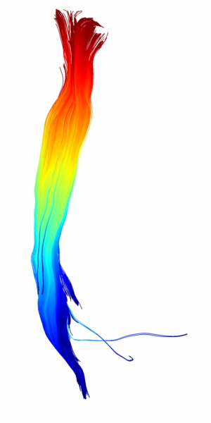
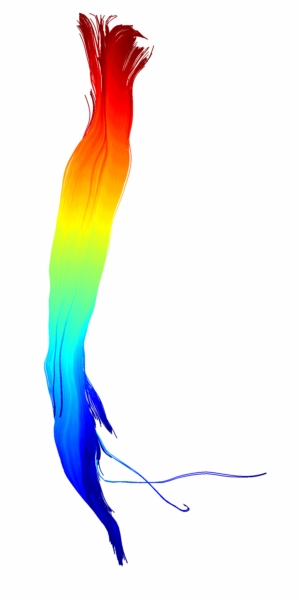
Like colors imply vertices whose associated DTI metrics will be averaged together to generate the along-tract mean cross-sectional estimates, and whose spatial positions will be averaged together to generate the mean tract geometry. The left panel shows the raw streamlines upon import, the center panel shows them after reorientation with trk_flip, and the right panel shows the difference if we prescribe an additional central correspondence point by flagging the [[tie_at_center|tie-at-center]] option to trk_interp. Again, color here is representing assumed correspondence, and not FA or direction.