Functional Reactive Programming
Functional Reactive Programming is an abstraction to define and operate with values that change over time.
Games and interactive software produce not a one-time output, but a continuous output over a period of time. Most of the time the output is determined also by input that is provided not all at once, but progressively during the execution.
Concepts in your program, such as the text of a widget, or the lives the player has left, change as the program moves forward. This is true, in general, for any part of your program that represents a changing state.
FRP is an abstraction to describe these changing values in terms of other changing values, so that all get updated when any of them is.
FRP is
an abstraction to define changing values in terms of other (changing) values.
This way, whenever a value changes, any other value that depends on it is also
updated. This is similar to a spreadsheet, in which changes to one cell affect
the values in other cells.
⭐ Fancy language for fancy people with glasses
FRP aims at being declarative as opposed to being operational. What this means is that you focus on how to define a value for all time, as opposed to deciding how to update it at any particular moment. Meaning, not action.
There are two ideas captured in FRP:
- How to define changing values (defined in terms of other changing values), and
- how to make those values depend on the past and the present.
FRP addresses the concerns above by introducing the time. A value that changes over time is a value that depends on time. A value that depends on the past depends on other values (or itself) at previous times. We call these changing values Signals:
Signal a = Time -> a
That is the basis of FRP. All the ideas, problems, optimisations, quirks, and papers work on variations of that idea, on giving them precise meaning under certain assumptions or in some environments, and on providing an efficient way of working with those abtractions.
🕙 Remember the time
The keyword in Functional Reactive Programming is not Reactive, it's Temporal. Reactivity is a nice side effect of the model (and it's also the intended usage), but the core idea is the introduction of time in the equations. You can do IO-based reactive programming in Haskell without time; in fact, many "FRP" implementations are actually F;RP, or just RP.
FRP is a temporal abstraction.
Let's imagine, for instance, that we want to describe continuous output. On your computer, at any point in time, a still image is rendered on the screen. To create an animation (as we do in games) we can just provide different pictures at different times.
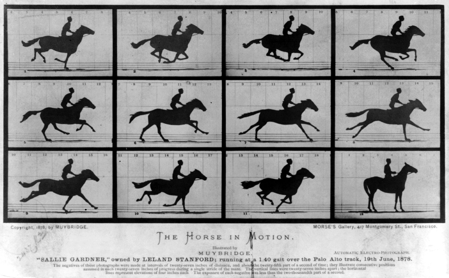
Photographer Eadwear Muybridge's pictures of The Horse in Motion, from
1878. Left, still images. Right, animation created from still images.
We could, of course, provide a list of frames and to be rendered at different times, but we could also describe the image in terms of time. For instance, a ball moving around the screen could be produced by rendering the still picture of a ball at a different position every time. The position could depend on the time:
rotatingBall :: Time -> Picture
rotatingBall time = translate stillBall (x,y)
 where x = centerX + rotationRadius * cos time
       y = centerY + rotationRadius * sin time
       -- Config settings
       rotationRadius = ... -- pixels
       stillBall      = ... -- picture of a ball
       translate      = ... -- picture function

Sure, continuous time can only be approximated, and the machine will use sampling, and time will (probably) have limited precision. What's interesting about this approach is that we could be as precise as we want with time, and the rotating ball would always have a precise meaning and a smooth animation (as smooth as the machine can provide). If we run it on a machine that is twice as fast, the animation still "work" perfectly fine because the actual time was used in the equations; it will simply render more precisely.
We can also apply time transformations to signals, for instance, we could delay the animation by just doing:
slowRotatingBall :: Signal Picture
slowRotatingBall time = rotatingBall (time / 2)
Definitions like this one show that we can go backwards and forwards in time, to roll time back, and rerun a specific part of the simulation slower and with more precision. Not only are we transforming time here, but we are also using a signal to create another signal.
📗 Vocabulary
Some FRP papers call these changing values Behaviors, and they also talk about events. Do not despair, we will get to that. In the current text you can think of Signals as equivalent to Behaviors.
Using this abstraction one can also model system input. For instance, the mouse is always at some position (as long as it is plugged), even if our system polls the mouse at a specific rate.
We can express equations based on this time-dependent mouse position, and thus focus on their true meaning.
ballAtMousePos :: Signal Picture
ballAtMousePos time = translate stillBall (mousePosition time)
 where -- Config settings
       stillBall = ... -- picture

Now we would have a ball that is always where the mouse is. We can even combine the two, and present a ball circling around the mouse:
ballAroundMousePos :: Signal Picture
ballAroundMousePos time = translate stillBall (x,y)
 where (mX, mY) = mousePos time
       x        = mX + rotationRadius * cos time
       y        = mY + rotationRadius * sin time
       -- Config settings
       stillBall = ... -- picture

Now, the above approach is all good, but it leaves a few open questions (it's ok if you haven't thought about them, we forgive you):
-
What happens if you ask for the mouse position 10 years in the future (or any time in the future)? Should the system hang while it waits? Does it even make sense to ask for that?
-
What happens if you ask for the mouse position 10 years in the past? Does it need to remember all the past? Even those moments when the system was not even being examined (in between frames)?
-
Functions that do IO in Haskell have IO signatures. From their types, it is clear that they actually depend on (or change) the state of the world. While
rotatingBallhas a pure meaning for all time (it does not depend on external input),ballAroundMousePosdoes, but both have the same type. What are the consequences and possible issues? How are testability, equational reasoning and referential transparency affected?
The first problem hints towards causality, the second to bounded memory and the third one to pure functions.
To address the previous concerns, we are going to move our reasoning one level up, from signals to functions that transform signals, and we will also introduce the following changes.
-
Input signals will now become function inputs. All signal functions will be pure, and we will have to explicitly connect these signal functions to the outside world.
-
Signals themselves will now be black boxes for us: we will be given combinators to create them and combine them, but we will have no ability to poll them at specific times. Time will always move towards the future.
-
Signal function combinators will ensure that not too much history is kept: most combinators will retain no history, and some will give us the ability to hold the current state for the future.
-
We will still have access to the total running time in a global signal function that we can always invoke:
time.
It's easier to think of signal functions as digital signal processing components that take an input signal and produce an output signal. Some of the types and combinators available are:
-
SF a bis the type of functions that take an input signal carrying values of typeaand return an output signal carrying values of typeb. -
arrapplies a pure Haskell function point-wise, or time-wise, just at every point in time, ignoring all history. -
(>>>)pipes signal functions. -
(&&&)pipes the same input to two SFs.
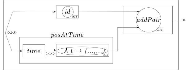
ballAroundMousePos :: SF (Double, Double) (Double, Double)
ballAroundMousePos =
  (arr id &&& posAtTime) >>> arr addPair

posAtTime :: SF a (Double, Double)
posAtTime =
  time >>> arr (\t -> (rotationRadius * cos t, rotationRadius * sin t))

addPair :: Num a => ((a, a), (a, a)) -> (a, a)
addPair ((x1,y1), (x2, y2)) = (x1 + x2, y1 + y2)
The difference here is that mousePos is not present. The mouse position is
given as a function input, so it is not necessarily IO. We could have called
the function ballAroundPos. There is no reference to the external world in
that implementation, and it could by used to move a ball around any signal that
contains a position.
Signal Functions can also be described using Arrow notation, as the following example depicts, which also renders simpler code in this case:
ballAroundMousePos :: SF (Double, Double) (Double, Double)
ballAroundMousePos = proc (centerX, centerY) -> do
  t <- time -< () -- to get the time we need to pass an input value
                  -- of any kind

  -- Displacement
  let dx = rotationRadius * cos t
      dy = rotationRadius * sin t

  returnA -< (centerX + dx, centerY + dy)
The way to understant the above code is:
-
Given an input signal, that carries a value, which is a tuple, whose components at any given time we call
centerXandcenterY, -
and given a signal, whose value at any time we call
t, which will always hold the current time -
let
dxbe defined by the formularotationRadius * cos t, and similarly fordy -
the output signal will always carry a tuple, whose components are
centerX + dxandcenterY + dy.
To execute this and connect it to the outisde world we need to gather an actual (mouse) position. We are also going to delay all rendering to outside the system, and simply produce a position where the ball should be. Let's look at a complete example that draws a circle around the wiimote "cursor".
main = do
  -- Initialise output
  SDL.init [InitVideo]
  SDL.setVideoMode width height 32 [SWSurface]

  -- Initialise clock
  curTime <- SDL.getTicks
  timer <- newIORef curTime

  -- Initialise input
  putStrLn "Initializing WiiMote. Please press 1+2 to connect."
  wm <- cwiidOpen
  case wm of
    Nothing      -> putStrLn "Could not connect" -- exit
    Just wiimote -> do
      putStrLn "Connected"
      -- Enable different sensors (15 = 1 + 2 + 4 + 8):
      -- 1 for status, 2 for buttons, 4 for accelerometers, and 8 for IR.
      cwiidSetRptMode wiimote 15


      -- FRP system
      Yampa.reactimate

         -- Connection to inputs
         (getIRCenterPos wiimote)
         (do dt <- getTimePassed timer
             pos <- getIRCenterPos wiimote
             return (Just (dt, pos)))

         -- Connection to outputs
         (\_ circlePos -> render circlePos)

         -- Actual transformation
         ballAroundMousePos

render :: (Int, Int) -> IO ()
render (x, y) = do
   screen <- getVideoSurface
   let format = surfaceGetPixelFormat screen
   white <- mapRGB format 255 255 255
   fillRect screen Nothing white

   filledCircle screen (fromIntegral x) (fromIntegral y) 30 (Pixel 0xFF0000FF)

SDL.flip screenThis approach enables writing time transformations that we know are safe to use given certain assumptions and separate their time-dependence. For instance, a useful transformation would be to add all the values that come in, multiplied by the time that has passed. This would result in a relatively simple approximation of the integral (which, in the limit, if we sampled infinitely fast, would be the actual integral).
We could then simulate physical processes very easily:
integral :: SF Double Double
integral = ...

fallingBall :: SF a (Int, Int)
fallingBall = constant 9.8 >>> integral >>> integral >>> arr (\y -> (512, y))
Or the equivalent formulation:
fallingBall :: SF a (Int, Int)
fallingBall = proc (_) -> do
  yVel <- integral -< 9.8
  yPos <- integral -< yVel
  returnA -< (512, yPos)
This falling ball now, as we can see, does not really depend on the nature
of the input: the acceleration (9.8) is integrated, the velocity is integrated,
and that is used as the y coordinate to represent a location on the screen.
Substitute aroundPos for fallingBall and you will see the following:

⭐ No tool can do all
Thinking in signal functions is, at least at first, very different from thinking in signals or just monadic FP. Personally, I do not advocate writing every part of every interactive program in FRP: it has a place, and it can be combined with other reactive libraries, with pure stateless functional programming, and with monadic IO.
Basic animations can indeed be very easy to describe and manipulate now. For instance, we can describe a function that zooms into a point by a factor as:
zoomAt :: (Double, Double) -> Double -> (Double, Double) -> (Double, Double)
zoomAt (centerX, centerY) factor (x, y) =
  (centerX + (x - centerX) * factor, centerY + (y - centerY) * factor)
And apply it to the previous animation seamlessly:
      -- FRP system
      Yampa.reactimate

         -- Input and output
         ...

         -- Actual transformation
         (ballAroundMousePos >>> arr (zoomAt (512, 384) 2))
PLACE FOR AN IMAGE
We can also very easily slow things down:
      -- FRP system
      Yampa.reactimate

         -- Input
         (getIRCenterPos wiimote)
         (do dt       <- getTimePassed timer
             pos      <- getIRCenterPos wiimote

             -- Adjust time
             slow     <- getWiimoteButtonA wiimote
             verySlow <- getWiimoteButtonB wiimote
             let dt' = if | verySlow  -> dt / 10
                          | slow      -> dt / 2
                          | otherwise -> dt

             return (Just (dt', pos)))

         -- Output
         ...

         -- Actual transformation
         ballAroundMousePos

getWiimoteButtonA :: CWiidCWiid -> IO Bool
getWiimoteButtonA wiimote = do
  allButtons <- cwiidGetBtnState wiimote
  return (cwiidIsBtnPushed allButtons cwiidBtnA)

getWiimoteButtonB :: CWiidCWiid -> IO Bool
getWiimoteButtonB  wiimote = ...
As you can see in the animation, the simulation slows down as mandated by the clock, affected by user input. Maybe the most important fact is that the number of frames per second of the execution is the same: it is not slowed down. It's just that time progresses in smaller steps.
A pure Yampa program slows down as the user depresses the left mouse
button (x2 slower) and the right mouse button (x10 slower). In this video, the
mouse is used instead of a wiimote, for visual feedback.
⭐ Extending Yampa
This code is based on the FRP implementation Yampa. In our games, we often extend Yampa to include new combinators. New extensions have to be written with care, to maintain causality and limit possible memory leaks. Feel free to do the same: if Yampa does not suit you completely, extend it. If the extension could be useful for others, send a bug report or a pull request via the github page.