As the machine learning community creates increasingly complex models and pervases areas of societal impact, we are struck with the problem of understanding decisions made by machine learning models without sacrificing their accuracy.
This repo contains some experiments with the concept of a local explainer, as presented by Ribeiro et. al in "Why Should I Trust You":Explainining the Predictions of Any Classifier. We explore the role of locality in the results with some toy examples, attempting to help answering the question: How can we be sure we can trust a local explainer?
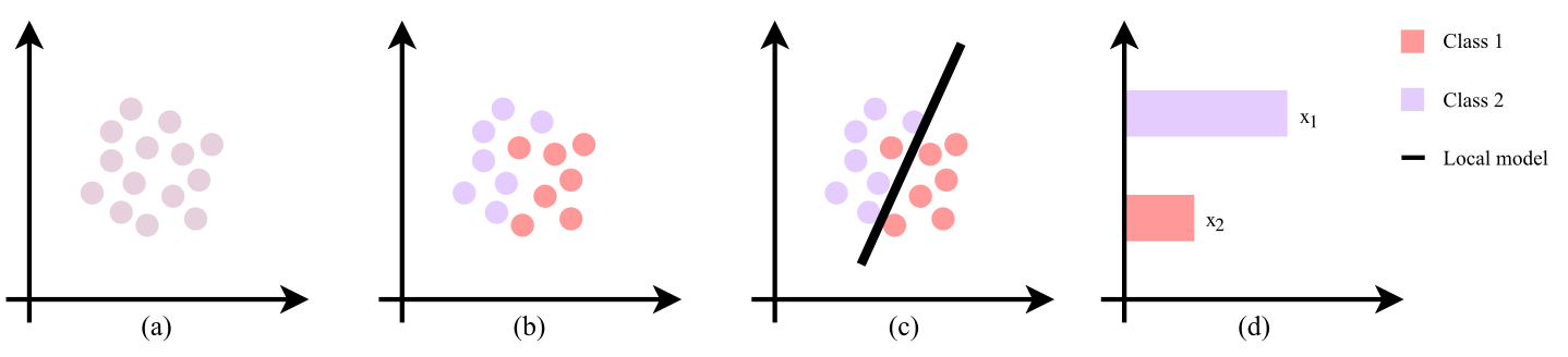
The local explainers, as implemented in LIME work in the following fashion. Given a decision d, a global model M we want to explain and a local model M' we want to use locally, we:
-
sample around a decision.
-
apply the global model to classify the generated samples.
-
apply the local model to the labeled samples.
-
extract information out of the local model to explain the decision.
These steps are illustrated in letters (a-d) in the figure bellow:
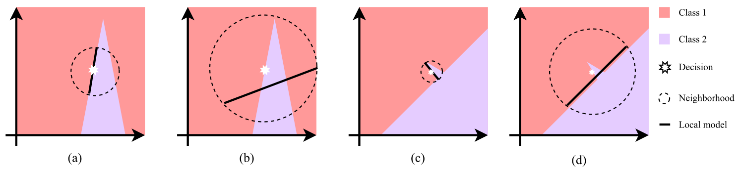
The possible problems you can have is that (as illustrated in the figure bellow):
-
Hard to know the how local the local model should be (a-b).
-
Multiple explanations may exist (c-d).
Notice that the steps in local explanation suggest a stack:
- A specific decision d, characterized by a vector of features.
- A global model M, which is the model we want to explain the decisions from.
- A local model M', which will be locally applied on the neighborhood of a decision.
- A sampler S, which will sample the neighborhood around a specific decision.
- A depicter D, which will present the local in a humanly understandable fashion.
In this repo we implement a logistic regression local model (M'), a gaussian sampler (S) and a bar chart depicter (D). We try to keep it generic. Notice that our stack only works for two labels and numerical features.
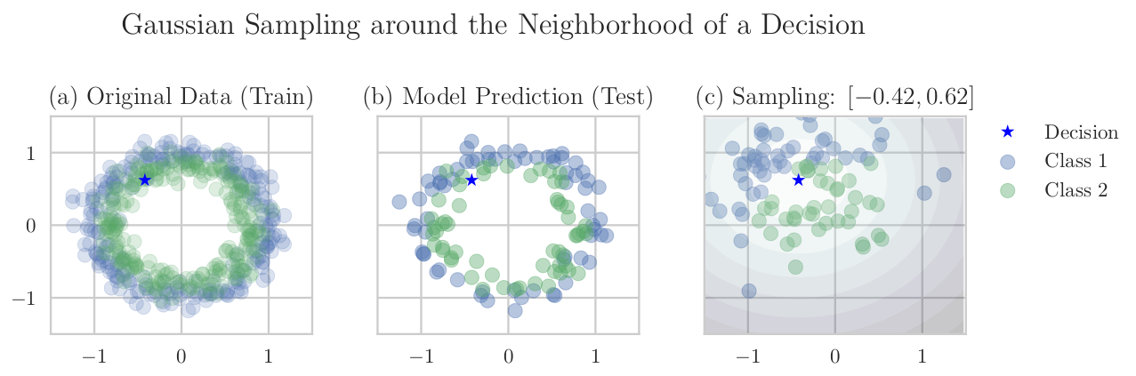
The sampler samples from a multivariate gaussian distribution N(d,Sigma), where the covariance the different random variables is 0. It also produces an exponential kernel, weighting the sampled distances. The steepness of the kernel l indicates how local the explanation is.
Sampling is as easy as:
decision = np.array([-0.42, 0.62])

sampler = GaussianExponentialSampler(X, ["Feature 1, Feature 2"], ["numerical", "numerical"],
                                     y, "Label", "Categorical",
                                     100, 0.05,
                                     rf.predict_proba)

sample_f, sample_l, weights = sampler.sample(decision)
An intuition behind sampling can be seen in the image bellow. Given the data in (a) we train the model in (b) and do the sampling in (c), labeling the instances with the model trained in (b).
Our explainer, or in other words, the local interpretable model that we fit in the more complex machine learning one is as weighted logistic regression.
Explaining is as easy as:
decision = np.array([-0.42, 0.62])

explainer = LogisticRegressionExplainer(sampler)

explainer.explain(decision)
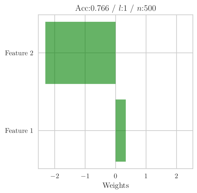
Our depicter saves or shows a simple bar chart with the weights of each one of the features. It can be tuned to plot on an axis/destination.
Depicting is as easy as:
destination = "./imgs/new_explanation.pdf"

exp_result = explainer.explanation_result()

depicter = my_depicter(destination)

depicter.depict(exp_result)
Check for yourself an example of an explanation using our simple depicter:
All of these things can be used together in the Explanation class, where you basically choose a sampler, an explainer and a depicter and explain away decisions. For example:
exp = Explanation(X_train, ["Feature 1", "Feature 2"], None,
                  y_train, "Label", None,
                  model=RandomForestClassifier(n_estimators=100),
                  explainer=LogisticRegressionExplainer,
                  sampler=GaussianExponentialSampler,
                  depicter=DepicterBarWeights,
                  destination=destination)

exp.sample_explain_depict(decision, depict=True)
We now start considering the problems that may appear as we locally explaining a complex model. Notice that we had two parameters in the sampler that were completely arbitrary. The sample size n and a measure of locality l, which in our specific case was related to the steepness of the exponential kernel.
It is not hard to prove with a toy example that both of these parameters have a huge impact in the local classifier that we are training. In the figures bellow we can see the variation of the explainer according to changes in the sample size n and in the measure of locality l.
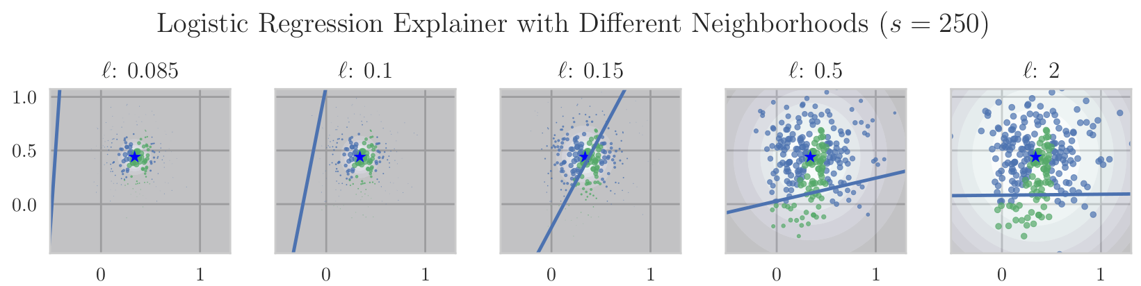
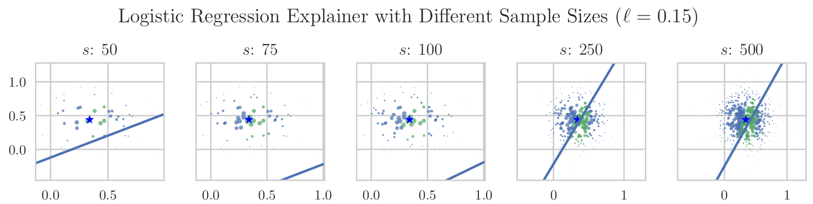
We can also inspect the mesh between the two variables and the parameters of the logistic regression, as it can be seen in the figure bellow.
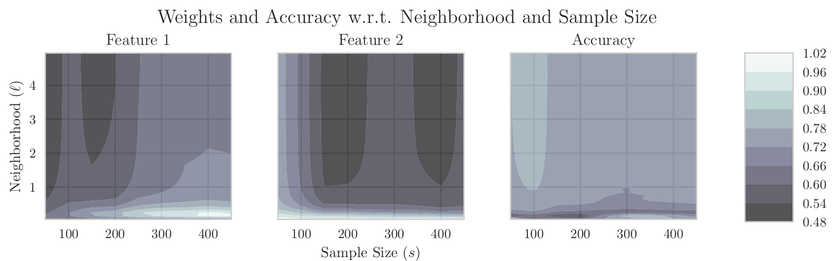
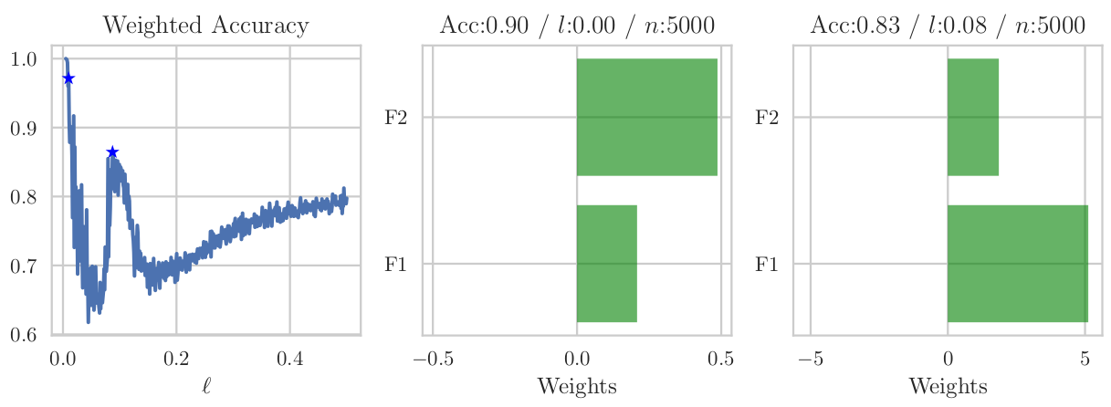
What this images show us is that we clearly have a problem in choosing this parameters. We implement a naïve and simple approach to deal with it. Given a large enough sample size (and we do not address that part of the problem), we want to find several different explanations with different measures of locality. We want to find this peaks in the accuracy, which represent this better explanations. As show in the figure bellow.
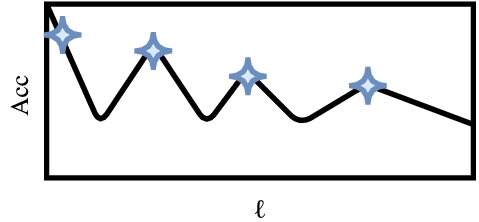
To do so we simply calculate the results for the explainer in a range of values, and then apply a simple peak detection algorithm to find different explanations with different localities. This is a wrapper around the Explanation class, and provides multiple explanations.
exp = RobustExplanation(X_train, ["F1", "F2"], None,
                        y_train, "Label", None,
                        model=RandomForestClassifier(n_estimators=100),
                        explainer=LogisticRegressionExplainer,
                        sampler=GaussianExponentialSampler,
                        depicter=DepicterBarWeights)

exp.sample_explain_depict(decision, 5, num_samples=5000, measure_min=0.005, measure_max=0.5, number_eval=500)
This can provide us with insight like the image bellow. We can get two different explanations with two different meanings.