🌎 Simple and fast watershed delineation in python.
Read the docs here 📖.
Hatari Labs - Elevation model conditioning and stream network delineation with python and pysheds 🇬🇧
Hatari Labs - Watershed and stream network delineation with python and pysheds 🇬🇧
Gidahatari - Delimitación de límite de cuenca y red hidrica con python y pysheds 🇪🇸
Earth Science Information Partners - Pysheds: a fast, open-source digital elevation model processing library 🇬🇧
Example data used in this tutorial are linked below:
- Elevation: elevation.tiff
- Terrain: impervious_area.zip
- Soil Polygons: soils.zip
Additional DEM datasets are available via the USGS HydroSHEDS project.
# Read elevation raster
# ----------------------------
from pysheds.grid import Grid

grid = Grid.from_raster('elevation.tiff')
dem = grid.read_raster('elevation.tiff')
Plotting code...
import numpy as np
import matplotlib.pyplot as plt
from matplotlib import colors
import seaborn as sns

fig, ax = plt.subplots(figsize=(8,6))
fig.patch.set_alpha(0)

plt.imshow(dem, extent=grid.extent, cmap='terrain', zorder=1)
plt.colorbar(label='Elevation (m)')
plt.grid(zorder=0)
plt.title('Digital elevation map', size=14)
plt.xlabel('Longitude')
plt.ylabel('Latitude')
plt.tight_layout()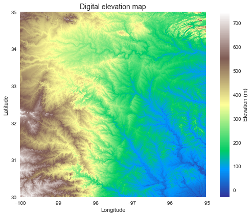
# Condition DEM
# ----------------------
# Fill pits in DEM
pit_filled_dem = grid.fill_pits(dem)

# Fill depressions in DEM
flooded_dem = grid.fill_depressions(pit_filled_dem)

# Resolve flats in DEM
inflated_dem = grid.resolve_flats(flooded_dem)# Determine D8 flow directions from DEM
# ----------------------
# Specify directional mapping
dirmap = (64, 128, 1, 2, 4, 8, 16, 32)
# Compute flow directions
# -------------------------------------
fdir = grid.flowdir(inflated_dem, dirmap=dirmap)Plotting code...
fig = plt.figure(figsize=(8,6))
fig.patch.set_alpha(0)

plt.imshow(fdir, extent=grid.extent, cmap='viridis', zorder=2)
boundaries = ([0] + sorted(list(dirmap)))
plt.colorbar(boundaries= boundaries,
             values=sorted(dirmap))
plt.xlabel('Longitude')
plt.ylabel('Latitude')
plt.title('Flow direction grid', size=14)
plt.grid(zorder=-1)
plt.tight_layout()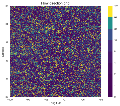
# Calculate flow accumulation
# --------------------------
acc = grid.accumulation(fdir, dirmap=dirmap)
Plotting code...
fig, ax = plt.subplots(figsize=(8,6))
fig.patch.set_alpha(0)
plt.grid('on', zorder=0)
im = ax.imshow(acc, extent=grid.extent, zorder=2,
               cmap='cubehelix',
               norm=colors.LogNorm(1, acc.max()),
               interpolation='bilinear')
plt.colorbar(im, ax=ax, label='Upstream Cells')
plt.title('Flow Accumulation', size=14)
plt.xlabel('Longitude')
plt.ylabel('Latitude')
plt.tight_layout()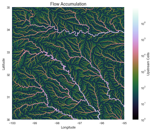
# Delineate a catchment
# ---------------------
# Specify pour point
x, y = -97.294, 32.737

# Snap pour point to high accumulation cell
x_snap, y_snap = grid.snap_to_mask(acc > 1000, (x, y))

# Delineate the catchment
catch = grid.catchment(x=x_snap, y=y_snap, fdir=fdir, dirmap=dirmap,
                       xytype='coordinate')

# Crop and plot the catchment
# ---------------------------
# Clip the bounding box to the catchment
grid.clip_to(catch)
clipped_catch = grid.view(catch)
Plotting code...
# Plot the catchment
fig, ax = plt.subplots(figsize=(8,6))
fig.patch.set_alpha(0)

plt.grid('on', zorder=0)
im = ax.imshow(np.where(clipped_catch, clipped_catch, np.nan), extent=grid.extent,
               zorder=1, cmap='Greys_r')
plt.xlabel('Longitude')
plt.ylabel('Latitude')
plt.title('Delineated Catchment', size=14)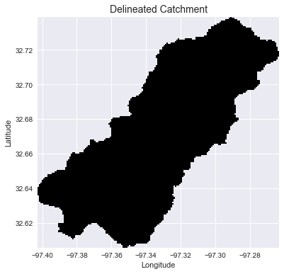
# Extract river network
# ---------------------
branches = grid.extract_river_network(fdir, acc > 50, dirmap=dirmap)
Plotting code...
sns.set_palette('husl')
fig, ax = plt.subplots(figsize=(8.5,6.5))

plt.xlim(grid.bbox[0], grid.bbox[2])
plt.ylim(grid.bbox[1], grid.bbox[3])
ax.set_aspect('equal')

for branch in branches['features']:
    line = np.asarray(branch['geometry']['coordinates'])
    plt.plot(line[:, 0], line[:, 1])

_ = plt.title('D8 channels', size=14)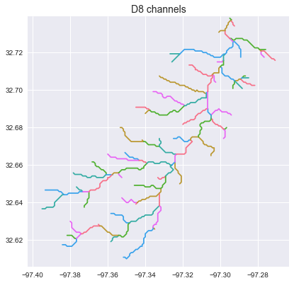
# Calculate distance to outlet from each cell
# -------------------------------------------
dist = grid.distance_to_outlet(x=x_snap, y=y_snap, fdir=fdir, dirmap=dirmap,
                               xytype='coordinate')
Plotting code...
fig, ax = plt.subplots(figsize=(8,6))
fig.patch.set_alpha(0)
plt.grid('on', zorder=0)
im = ax.imshow(dist, extent=grid.extent, zorder=2,
               cmap='cubehelix_r')
plt.colorbar(im, ax=ax, label='Distance to outlet (cells)')
plt.xlabel('Longitude')
plt.ylabel('Latitude')
plt.title('Flow Distance', size=14)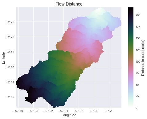
# Combine with land cover data
# ---------------------
terrain = grid.read_raster('impervious_area.tiff', window=grid.bbox,
                           window_crs=grid.crs, nodata=0)
# Reproject data to grid's coordinate reference system
projected_terrain = terrain.to_crs(grid.crs)
# View data in catchment's spatial extent
catchment_terrain = grid.view(projected_terrain, nodata=np.nan)
Plotting code...
fig, ax = plt.subplots(figsize=(8,6))
fig.patch.set_alpha(0)
plt.grid('on', zorder=0)
im = ax.imshow(catchment_terrain, extent=grid.extent, zorder=2,
               cmap='bone')
plt.colorbar(im, ax=ax, label='Percent impervious area')
plt.xlabel('Longitude')
plt.ylabel('Latitude')
plt.title('Percent impervious area', size=14)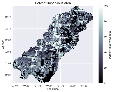
# Convert catchment raster to vector and combine with soils shapefile
# ---------------------
# Read soils shapefile
import pandas as pd
import geopandas as gpd
from shapely import geometry, ops
soils = gpd.read_file('soils.shp')
soil_id = 'MUKEY'
# Convert catchment raster to vector geometry and find intersection
shapes = grid.polygonize()
catchment_polygon = ops.unary_union([geometry.shape(shape)
                                     for shape, value in shapes])
soils = soils[soils.intersects(catchment_polygon)]
catchment_soils = gpd.GeoDataFrame(soils[soil_id],
                                   geometry=soils.intersection(catchment_polygon))
# Convert soil types to simple integer values
soil_types = np.unique(catchment_soils[soil_id])
soil_types = pd.Series(np.arange(soil_types.size), index=soil_types)
catchment_soils[soil_id] = catchment_soils[soil_id].map(soil_types)
Plotting code...
fig, ax = plt.subplots(figsize=(8, 6))
catchment_soils.plot(ax=ax, column=soil_id, categorical=True, cmap='terrain',
                     linewidth=0.5, edgecolor='k', alpha=1, aspect='equal')
ax.set_xlim(grid.bbox[0], grid.bbox[2])
ax.set_ylim(grid.bbox[1], grid.bbox[3])
plt.xlabel('Longitude')
plt.ylabel('Latitude')
ax.set_title('Soil types (vector)', size=14)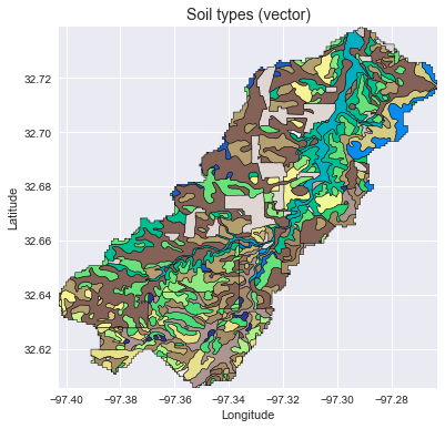
soil_polygons = zip(catchment_soils.geometry.values, catchment_soils[soil_id].values)
soil_raster = grid.rasterize(soil_polygons, fill=np.nan)
Plotting code...
fig, ax = plt.subplots(figsize=(8, 6))
plt.imshow(soil_raster, cmap='terrain', extent=grid.extent, zorder=1)
boundaries = np.unique(soil_raster[~np.isnan(soil_raster)]).astype(int)
plt.colorbar(boundaries=boundaries,
             values=boundaries)
ax.set_xlim(grid.bbox[0], grid.bbox[2])
ax.set_ylim(grid.bbox[1], grid.bbox[3])
plt.xlabel('Longitude')
plt.ylabel('Latitude')
ax.set_title('Soil types (raster)', size=14)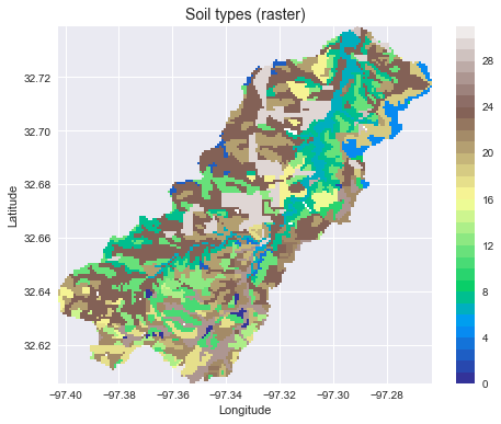
- Hydrologic Functions:
flowdir: Generate a flow direction grid from a given digital elevation dataset.catchment: Delineate the watershed for a given pour point (x, y).accumulation: Compute the number of cells upstream of each cell; if weights are given, compute the sum of weighted cells upstream of each cell.distance_to_outlet: Compute the (weighted) distance from each cell to a given pour point, moving downstream.distance_to_ridge: Compute the (weighted) distance from each cell to its originating drainage divide, moving upstream.compute_hand: Compute the height above nearest drainage (HAND).stream_order: Compute the (strahler) stream order.extract_river_network: Extract river segments from a catchment and return a geojson object.extract_profiles: Extract river segments and return a list of channel indices along with a dictionary describing connectivity.cell_dh: Compute the drop in elevation from each cell to its downstream neighbor.cell_distances: Compute the distance from each cell to its downstream neighbor.cell_slopes: Compute the slope between each cell and its downstream neighbor.fill_pits: Fill single-celled pits in a digital elevation dataset.fill_depressions: Fill multi-celled depressions in a digital elevation dataset.resolve_flats: Remove flats from a digital elevation dataset.detect_pits: Detect single-celled pits in a digital elevation dataset.detect_depressions: Detect multi-celled depressions in a digital elevation dataset.detect_flats: Detect flats in a digital elevation dataset.
- Viewing Functions:
view: Returns a "view" of a dataset defined by the grid's viewfinder.clip_to: Clip the viewfinder to the smallest area containing all non- null gridcells for a provided dataset.nearest_cell: Returns the index (column, row) of the cell closest to a given geographical coordinate (x, y).snap_to_mask: Snaps a set of points to the nearest nonzero cell in a boolean mask; useful for finding pour points from an accumulation raster.
- I/O Functions:
read_ascii: Reads ascii gridded data.read_raster: Reads raster gridded data.from_ascii: Instantiates a grid from an ascii file.from_raster: Instantiates a grid from a raster file or Raster object.to_ascii: Write grids to delimited ascii files.to_raster: Write grids to raster files (e.g. geotiff).
pysheds supports both D8 and D-infinity routing schemes.
pysheds currently only supports Python 3.
You can install pysheds using pip:
$ pip install pyshedsFirst, add conda forge to your channels, if you have not already done so:
$ conda config --add channels conda-forgeThen, install pysheds:
$ conda install pyshedsFor the bleeding-edge version, you can install pysheds from this github repository.
$ git clone https://github.com/mdbartos/pysheds.git
$ cd pysheds
$ python setup.py install
or
$ git clone https://github.com/mdbartos/pysheds.git
$ cd pysheds
$ pip install .
Performance benchmarks on a 2015 MacBook Pro (M: million, K: thousand):
| Function | Routing | Number of cells | Run time |
|---|---|---|---|
flowdir |
D8 | 36M | 1.14 [s] |
flowdir |
DINF | 36M | 7.01 [s] |
flowdir |
MFD | 36M | 4.21 [s] |
accumulation |
D8 | 36M | 3.44 [s] |
accumulation |
DINF | 36M | 14.9 [s] |
accumulation |
MFD | 36M | 32.5 [s] |
catchment |
D8 | 9.76M | 2.19 [s] |
catchment |
DINF | 9.76M | 3.5 [s] |
catchment |
MFD | 9.76M | 17.1 [s] |
distance_to_outlet |
D8 | 9.76M | 2.98 [s] |
distance_to_outlet |
DINF | 9.76M | 5.49 [s] |
distance_to_outlet |
MFD | 9.76M | 13.1 [s] |
distance_to_ridge |
D8 | 36M | 4.53 [s] |
distance_to_ridge |
DINF | 36M | 14.5 [s] |
distance_to_ridge |
MFD | 36M | 31.3 [s] |
hand |
D8 | 36M total, 730K channel | 12.3 [s] |
hand |
DINF | 36M total, 770K channel | 15.8 [s] |
hand |
MFD | 36M total, 770K channel | 29.8 [s] |
stream_order |
D8 | 36M total, 1M channel | 3.99 [s] |
extract_river_network |
D8 | 36M total, 345K channel | 4.07 [s] |
extract_profiles |
D8 | 36M total, 345K channel | 2.89 [s] |
detect_pits |
N/A | 36M | 1.80 [s] |
detect_flats |
N/A | 36M | 1.84 [s] |
fill_pits |
N/A | 36M | 2.52 [s] |
fill_depressions |
N/A | 36M | 27.1 [s] |
resolve_flats |
N/A | 36M | 9.56 [s] |
cell_dh |
D8 | 36M | 2.34 [s] |
cell_dh |
DINF | 36M | 4.92 [s] |
cell_dh |
MFD | 36M | 30.1 [s] |
cell_distances |
D8 | 36M | 1.11 [s] |
cell_distances |
DINF | 36M | 2.16 [s] |
cell_distances |
MFD | 36M | 26.8 [s] |
cell_slopes |
D8 | 36M | 4.01 [s] |
cell_slopes |
DINF | 36M | 10.2 [s] |
cell_slopes |
MFD | 36M | 58.7 [s] |
Speed tests were run on a conditioned DEM from the HYDROSHEDS DEM repository
(linked above as elevation.tiff).
If you have used this codebase in a publication and wish to cite it, consider citing the zenodo repository:
@misc{bartos_2020,
    title  = {pysheds: simple and fast watershed delineation in python},
    author = {Bartos, Matt},
    url    = {https://github.com/mdbartos/pysheds},
    year   = {2020},
    doi    = {10.5281/zenodo.3822494}
}