
Numerical experiments with stochastic differential equations in Haskell
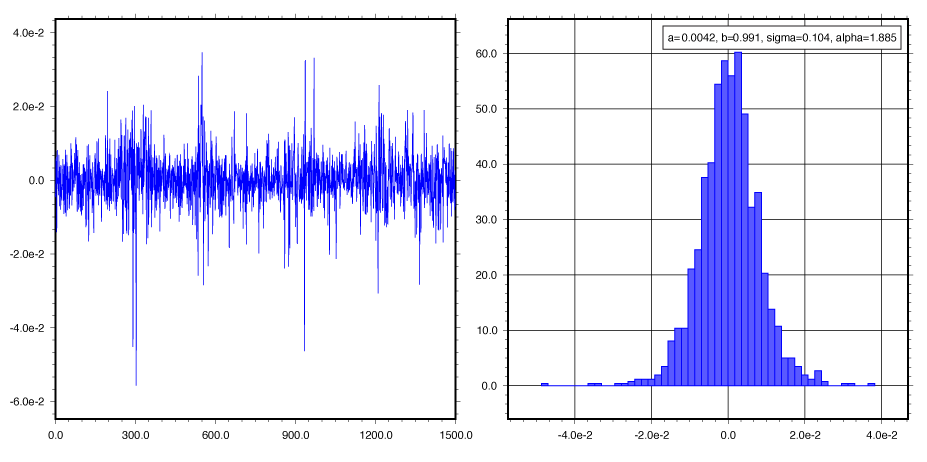
In the figure above, a sample path (left) and histogram of the variable y_t as formulated in the following stochastic volatility model [1]:
y_t = a exp(x_t / 2) v_t           (1)

x_t = b x_{t-1} + sigma u_t
where
u_t ~ N(0, 1)

v_t ~ S_alpha(1, 0, 0).
S_alpha(1, 0, 0) denotes the Levy-stable distribution with parameters (alpha, 1), where 0 < alpha <= 2. The special cases alpha=1 and alpha=2 correspond to the Cauchy-Lorentz and Gaussian distributions, respectively. Values of the alpha parameter smaller than 2 result in sudden large deviations typical of "heavy tailed" distributions, which can be used to model shocks or phase changes in underlying phenomena.
The library relies on mwc-probability for its primitive sampling functionality, and on the StateT monad transformer.
newtype Transition m a = Trans { runTrans :: Gen (PrimState m) -> StateT a m a }
The SDE integration process can be seen as an interleaved sequence of random sampling and state transformation. Formally, we are sampling independent increments (a Wiener process) of the state variable. The transition function, shown below, declares one such stochastic transion:
transition :: Monad m => Prob m a -> (b -> a -> b) -> Transition m b
transition msf f = Trans $ \g -> do
  x <- get
  w <- lift $ sample msf g
  let z = f x w
  put z
  return z
For example, the stochastic volatility model shown in the beginning can be implemented as follows :
data SV1 = SV1 {sv1x :: Double, sv1y :: Double} deriving (Eq, Show)

stochVolatility1 :: PrimMonad m => Double -> Double -> Double -> Double -> Transition m SV1
stochVolatility1 a b sig alpha = transition randf f where
  randf = (,) <$> normal 0 1
              <*> alphaStable100 alpha
  f (SV1 x _) (ut, vt) = let xt = b * x + sig * ut
                             yt = a * exp (xt / 2) * vt
                         in SV1 xt yt
This formulation lets the library user focus exclusively on the mathematical details of the model she wishes to simulate.
Once the stochastic model is written in terms of the Transition type, we may simulate a sample path with a runner function such as the following:
samplePathSDE :: Monad m => Int -> Transition m s -> s -> Gen (PrimState m) -> m [s]
samplePathSDE n sde x0 g = evalStateT (replicateM n (runTrans sde g)) x0
The random generator g :: Gen (PrimState m) can be instantiated either with create (which by default will reuse the seed therefore producing the same random sequence at every call), or within the bracket withSystemRandom . asIOGen, which taps from the operating system's random generator. Please refer to the documentation of mwc-probability for details.
Currently, only the Euler-Maruyama integration method has been implemented (the sampleSDE function shown above); this works for some models but is inaccurate and unstable for others; therefore one of the next development goals will be to include higher-order integration schemes such as those shown in Wilkie [2].
[1] Li, K. and Oestergaard, J. - Inference for a stochastic volatility model using MCMC with ABC-SMC approximation
[2] Wilkie, J. - Numerical methods for stochastic differential equations (https://arxiv.org/abs/quant-ph/0407039)