pyReef-Core is a deterministic, one-dimensional (1-D) numerical model, that simulates the vertical coralgal growth patterns observed in a drill core, as well as the physical, environmental processes that effect coralgal growth. The model is capable of integrating ecological processes like coralgal community interactions over centennial-to-millennial scales using predator-prey or Generalised Lotka-Volterra Equations.

Schematic figure of a hypothetical reef with transitions from shallow to deep assemblages occurring down-core, illustrating growth-form responses of corals to environmental forcing including light, sea level changes (sl), uplift and subsidence (u/s), hydrodynamic energy (w wave conditions and c currents), nutrients input nu, ocean temperature (T) and acidity (pH), karstification (k) and sediment flux.
- Generalized Lotka-Volterra model
- Communities rate and community matrix
- Carbonate production
- Model workflow
- Installation
- Usage
- Input file structure
- Examples
The most common models of communities evolution in ecological modeling are the predator-prey Lotka-Volterra (LV) equation and its modifications.
From LV equations, one can formulate the Generalized Lotka-Volterra (GLV) equation that allows unlimited number of communities and different types of interactions among communities. The GLV equation is mainly formed by two parts, the logistic growth/decay of a communities and its interaction with the other communities,

where 


where 


To solve the ODEs, the user needs to define several initial conditions:
- the initial community population number
- the intrinsic rate of a population community
- the interaction coefficients among the communities association


Several other inputs are required and will need to be set in the XmL inputfile. An example of such file is provided in the Tests folder and all the options are explained in the Input file structure.
The mathematical model for the communities population evolution results in a set of differential equations (ODEs), one for each communities associations modeled. The Runge-Kutta-Fehlberg method (RKF45 or Fehlberg as defined in the odespy library) is used to solve the GLV ODE system.
Once a community association population is computed, carbonate production is calculated using a carbonate production factor. Production factors are specified for the maximum population, and linearly scaled to the actual population following the relation

where 


which gives:

We define the maximum carbonate production rate (m/y) for each community in the XmL input file.

Illustration outlining PyReef-Core workflow (left) and of the resulting simulated core (right). First boundary conditions for sea level, sediment input, tectonics, temperature, pH, nutrients and flow velocity are set, which describes their relationship to either depth or time. The boundary conditions are used to establish the environment factor fenv which describes the proportion of the maximum growth rate that an assemblage can achieve, depending on whether the environmental conditions exceed the optimal conditions for growth. The environment factor is set to scale the Malthusian parameter, which is in turn used as input in the GLVE equations to determine assemblage populations. Larger assemblage populations contribute to a faster rate of vertical accretion (here referred to as carbonate production). In case of subaerial exposure, karstification might occur. At the end of the timestep, boundary conditions are updated and the process is repeated.
The code is available from our github page and can be obtained either from this page or using git
git clone https://github.com/pyReef-model/pyReefCore.git
Once donwloaded, navigate to the pyReefCore folder and run the following command:
pip install -e /workspace/volume/pyReefCore/
The code is available from Docker Hub at pyreefmodel/pyreef-Docker and can be downloaded using Kitematic. Examples are provided in the Tests folder and are ran through IPython Notebooks.
pyReef-Core can be used from an IPython notebook or a python script directly. An example of functions available is provided below:
%matplotlib inline

import numpy as np
import cmocean as cmo
import matplotlib.pyplot as plt

%config InlineBackend.figure_format = 'svg'

from pyReefCore.model import Model

# Initialise model
reef = Model()

# Define the XmL input file
reef.load_xml('input.xml')

# Visualise initial setting parameters
reef.core.initialSetting(size=(10,4), fname='input')

# Run to a given time (for example 500 years)
reef.run_to_time(500.,showtime=500.,verbose=False)

# Define a colorscale to display the core
# Some colormaps are available from the following link:
# http://matplotlib.org/examples/color/colormaps_reference.html
from matplotlib.cm import terrain, plasma
nbcolors = len(reef.core.coralH)+10
colors = terrain(np.linspace(0, 1, nbcolors))
nbcolors = len(reef.core.layTime)+3
colors2 = plasma(np.linspace(0, 1, nbcolors))

# Plot evolution of communities population with time
reef.plot.communityTime(colors=colors, size=(10,4), font=8, dpi=100,fname='apop_t.pdf')

# Plot evolution of communities population with depth
reef.plot.communityDepth(colors=colors, size=(10,4), font=8, dpi=100, fname ='apop_d.pdf')

# Plot temporal evolution of accommodation and core thickness
reef.plot.accommodationTime(size=(10,4), font=8, dpi=100, fname ='acc_t.pdf')

# Plot coral facies distribution, assemblages as a synthetic core
reef.plot.drawCore(lwidth = 3, colsed=colors, coltime = colors2, size=(10,8), font=8, dpi=380,
figname=('core.pdf'), filename='core.csv', sep='\t')- Time structure
- Habitats structure
- Sea-level structure
- Temperature structure
- pH structure
- Nutrients structure
- Flow structure
- Sediment structure
- Environmental structure
- Output folder structure
<?xml version="1.0" encoding="UTF-8"?>
<pyreefcore xmlns:xsi="http://www.w3.org/2001/XMLSchema-instance">REQUIRED
  <!-- Simulation time structure -->
  <time>
    <!-- Simulation start time [a] -->
    <start>-140000.</start>
    <!-- Simulation end time [a] -->
    <end>0.</end>
    <!-- Time step for carbonate module [a] -->
    <tcarb>5.</tcarb>
    <!-- Display interval [a] -->
    <display>100.</display>
    <!-- Stratigraphic layer interval [a] -->
    <laytime>25.</laytime>
</time>REQUIRED
  <!-- Community definition, initial population and position. -->
  <habitats>
    <!-- Initial depth relative to sea-level at start time [m].
         Note: positive when below sea-level. -->
    <depth>25.</depth>
    <!-- Number of communities to define. -->
    <communityNb>3</communityNb>
    <!-- Maximum population number. -->
    <maxPopulation>10</maxPopulation>
    <!-- Turn-on criterion. Population growth only occurs when the
         optimum is met. This reflects the notion that reef ‘turn on’
         events occur because of a confluence of optimal conditions [0,1]. -->
    <facOpt>0.9</facOpt>
    <!-- Karstification rates in subaerial domain [m/y]. -->
    <karstRate>0.07e-3</karstRate>

    <!-- Community definition -->
    <community>
      <!-- Community name needs to be lower than 10 characters -->
      <!-- Shallow assemblage -->
      <name>shallow</name>
      <!-- Definition of intrinsic rate of increase/decrease of the
           considered population of community (Malthusian parameter). -->
      <malthus>0.004</malthus>
      <!-- Initial population number for considered community. -->
      <population>0.</population>
      <!-- Community maximum production rate for considered community [m/y]. -->
      <production>0.011</production>
    </community>

    <!-- Community definition -->
    <!-- Medium assemblage (6-20 m), similar to tabular/branching coral facies of Indo-Pacific.
         Represents growth at beginning of 'catch-up' reef -->
    <community>
      <!-- Community name needs to be lower than 10 characters -->
      <name>moderate deep</name>
      <!-- Definition of intrinsic rate of increase/decrease of the
           considered population of community (Malthusian parameter). -->
      <malthus>0.004</malthus>
      <!-- Initial population number for considered community. -->
      <population>0.</population>
      <!-- Community maximum production rate for considered community [m/y]. -->
      <production>0.012</production>
    </community>

    <!-- Community definition -->
    <!-- Deep assemblage (20-30 m), of domal/branching and encrusting types.
         Represents reef-drowning events -->
    <community>
      <!-- Community name needs to be lower than 10 characters -->
      <name>deep</name>
      <!-- Definition of intrinsic rate of increase/decrease of the
           considered population of community (Malthusian parameter). -->
      <malthus>0.004</malthus>
      <!-- Initial population number for considered community. -->
      <population>0.</population>
      <!-- Community maximum production rate for considered community [m/y]. -->
      <production>0.009</production>
    </community>

    <!-- Community matrix representing the interactions between communities.
         αij is the interaction coefficient among the communities association i and j ,
         (a particular case is αii, the interaction of one communities association with itself).

         Example on how to define the following community matrix of αij coefficients
         with i the column and j the row:
                     -0.0005  -0.0001   0.
                     -0.0001  -0.0005  -0.0001
                      0.      -0.0001  -0.0005
    -->
    <communityMatrix>
      <!-- Interaction for communities 1 -->
      <value col="0" row="0">-0.0005</value>
      <value col="1" row="0">-0.0001</value>
      <value col="2" row="0">0.</value>

      <!-- Interaction for communities 2 -->
      <value col="0" row="1">-0.0001</value>
      <value col="1" row="1">-0.0005</value>
      <value col="2" row="1">-0.0001</value>

      <!-- Interaction for communities 3 -->
      <value col="0" row="2">0.0</value>
      <value col="1" row="2">-0.0001</value>
      <value col="2" row="2">-0.0005</value>
    </communityMatrix>
</habitats>OPTIONAL
  <!-- Sea-level structure
    The following methods can be used:
      - a constant sea-level position for the entire simulation [m]
      - a sea-level fluctuations curve (defined in a file)
  -->
  <sea>
    <!-- Constant sea-level value [m] -->
    <val>0.</val>
    <!-- Sea-level curve - (optional). The file is made of 2 columns:
      - first column: the time in year (increasing order)
      - second column: the sea-level position for the considered time [m]
       For any given time in the simulation the sea-level is obtained by linear interpolation
    -->
    <curve>data/grantetal.csv</curve>
</sea>OPTIONAL
  <!-- Uplift/subsidence structure
    The following methods can be used:
      - a constant subsidence/uplift rate for the entire simulation [m/y]
      - a subsidence/uplift curve (defined in a file)
  -->
  <tec>
    <!-- Constant tectonic value [m/y] -->
    <val>-0.1e-3</val>
    <!-- Tectonic curve - (optional). The file is made of 2 columns:
      - first column: the time in year (increasing order)
      - second column: the tectonic rate for the considered time [m/y]
       For any given time in the simulation the tectonic rate is obtained by linear interpolation
    <curve>data/tectonics.csv</curve>
    -->
</tec>OPTIONAL
  <!-- Temperature structure - (optional). -->
  <temp>
    <!-- Defined in a file made of 2 columns:
      - first column: the time in year (increasing order)
      - second column: number ranging between [0,1]
      The second column estimates the effect of temperature on all communities,
      where 0 inhibitory effects (either too high or too low temperature) and 1 corresponds to
      favourable conditions. -->
    <curve>data/temperature.csv</curve>
</temp>OPTIONAL
  <!-- pH structure - (optional). -->
  <pH>
    <!-- Defined in a file made of 2 columns:
      - first column: the time in year (increasing order)
      - second column: number ranging between [0,1]
      The second column estimates the effect of pH on all communities,
      where 0 inhibitory effects (either too high or too low pH) and 1 corresponds to
      favourable conditions. -->
    <curve>data/pH.csv</curve>
</pH>OPTIONAL
  <!-- Nutrients structure - (optional). -->
  <Nu>
    <!-- Defined in a file made of 2 columns:
      - first column: the time in year (increasing order)
      - second column: number ranging between [0,1]
      The second column estimates the effect of pH on all communities,
      where 0 inhibitory effects (either too high or too low Nutrients) and 1 corresponds to
      favourable conditions. -->
    <curve>data/pH.csv</curve>
</Nu>OPTIONAL
  <!-- Ocean flow structure
    The following methods can be used:
      - a constant flow velocity for the entire simulation [m/d]
      - a flow velocity fluctuations curve (defined in a file)
      - a flow velocity function dependent of water depth
  -->
  <flow>
    <!-- Constant velocity value [m/d] -->
    <!--val>0.</val-->
    <!-- Flow velocity curve - (optional). The file is made of 2 columns:
      - first column: the time in year (increasing order)
      - second column: the flow velocity for the considered time [m/d]
       For any given time in the simulation the flow velocity is obtained by linear interpolation
    -->
    <!--curve>data/flow.csv</curve-->
    <!-- Flow velocity function - (optional).
       For any given time in the simulation the flow velocity is obtained from water depth evaluation
       using either :
           - a linear function (y=ax+b) or
          - an exponential decay function based on 3 points fitting.
       The points need to be specify below:
    -->
    <function>
      <!--linear>
        <fmax>20.</fmax>
        <a>-0.33</a>
        <b>20</b>
      </linear-->
      <expdecay>
      <!-- Values from Sebens et al., 2003 -->
        <!-- X coordinates (velocity) m/s -->
        <fdvalue col="0" row="0">0.03</fdvalue>
        <fdvalue col="1" row="0">0.05</fdvalue>
        <fdvalue col="2" row="0">0.06</fdvalue>
        <fdvalue col="3" row="0">0.13</fdvalue>
        <fdvalue col="4" row="0">0.25</fdvalue>
        <!-- Y coordinates (depth) m -->
        <fdvalue col="0" row="1">25</fdvalue>
        <fdvalue col="1" row="1">15.</fdvalue>
        <fdvalue col="2" row="1">10.</fdvalue>
        <fdvalue col="3" row="1">3.</fdvalue>
        <fdvalue col="4" row="1">0.</fdvalue>
      </expdecay>
    </function>
</flow>OPTIONAL
  <!-- Siliciclastic input structure
    The following methods can be used:
      - a constant sediment influx for the entire simulation [m/y]
      - a sediment influx fluctuations curve (defined in a file)
      - a sediment influx function dependent of water depth
  -->
  <sedinput>
    <!-- Constant velocity value [m/s] -->
    <!--val>0.</val-->
    <!-- Flow velocity curve - (optional). The file is made of 2 columns:
      - first column: the time in year (increasing order)
      - second column: the flow velocity for the considered time [m/s]
       For any given time in the simulation the flow velocity is obtained by linear interpolation
    -->
    <!--curve>data/sedinput.csv</curve-->
    <!-- Sediment input function - (optional).
       For any given time in the simulation the sediment input is obtained from water depth evaluation
       using either :
           - a linear function (y=ax+b) or
          - an exponential decay function based on 3 points fitting.
       The points need to be specify below:
    -->
    <function>
      <!-- Windward curve as 4x less sedimentation than leeward-->
      <linear>
        <dmax>30.</dmax>
        <a>15000</a>   <!-- Max Sed = 0.008 m/y, intercepts = (0.004,0) (0.008,30)-->
        <b>-15.</b>
      </linear>
      <?ignore
      <expdecay>
        <!-- X coordinates (sediment input) m/d -->
        <sdvalue col="0" row="0">1.e-7</sdvalue>
        <sdvalue col="1" row="0">5.e-7</sdvalue>
        <sdvalue col="2" row="0">1.e-6</sdvalue>
        <!-- Y coordinates (depth) m -->
        <sdvalue col="0" row="1">20</sdvalue>
        <sdvalue col="1" row="1">3.</sdvalue>
        <sdvalue col="2" row="1">0.</sdvalue>
      </expdecay>
      ?>
    </function>
</sedinput>Using the XmL input file you will be able to calibrate the environmental threshold functions for different assemblages. Figure below shows an example of calibration for shallow, moderate-deep and deep assemblages characteristic of a synthetic exposed margin. The x-axis indicates the limitation on maximum vertical accretion for conditions outside the optimal.

REQUIRED
  <!-- Combining environmental parameters and carbonate production structure.
    The influence functions for each environmental factor (water depth, flow velocity, and sediment input)
    are used to model the interaction between communities and their environment. For the sake of simplicity,
    these functions have a trapezoidal shape that the user can define through four points [A,B,C,D].
    A is the minimal value below which the communities cannot live. Points B and C define the range where
    the community has the best conditions for development. D is the value over which the communities cannot live.
    The function is linearly interpolated between these points.
    This is optional.
  -->
  <envishape>

    <!-- Definition of water depth shape function influencing each community [m].
                  Min.[A]    Opt.1 [B]    Opt.2 [C]    Max. [D]
    Community1     0.           0.           6.          12.
    Community2     4.           6.          20.          22.
    Community3     18.          20.         30.          32.
    -->
    <depthshape>
      <!-- Definition of point A, B, C and D for first community -->
      <dvalue col="0" row="0">0.</dvalue>
      <dvalue col="1" row="0">0.</dvalue>
      <dvalue col="2" row="0">6.</dvalue>
      <dvalue col="3" row="0">12.</dvalue>
      <!-- Definition of point A, B, C and D for second community -->
      <dvalue col="0" row="1">4.</dvalue>
      <dvalue col="1" row="1">6.</dvalue>
      <dvalue col="2" row="1">20.</dvalue>
      <dvalue col="3" row="1">22.</dvalue>
      <!-- Definition of point A, B, C and D for third community -->
      <dvalue col="0" row="2">18.</dvalue>
      <dvalue col="1" row="2">20.</dvalue>
      <dvalue col="2" row="2">30.</dvalue>
      <dvalue col="3" row="2">32.</dvalue>
    </depthshape>

    <!-- Definition of flow velocity shape function influencing each community [m/s].
                        Min.[A]    Opt.1 [B]    Opt.2 [C]    Max. [D]
            Community1   0.05       0.06         0.25         0.3
            Community2   0.         0.05         0.09         0.12
            Community3   0.         0.           0.04         0.08
    -->
    <flowshape>
      <!-- Definition of point A, B, C and D for first community -->
      <fvalue col="0" row="0">0.05</fvalue>
      <fvalue col="1" row="0">0.06</fvalue>
      <fvalue col="2" row="0">0.25</fvalue>
      <fvalue col="3" row="0">0.3</fvalue>
      <!-- Definition of point A, B, C and D for second community -->
      <fvalue col="0" row="1">0.</fvalue>
      <fvalue col="1" row="1">0.05</fvalue>
      <fvalue col="2" row="1">0.09</fvalue>
      <fvalue col="3" row="1">0.12</fvalue>
      <!-- Definition of point A, B, C and D for third community -->
      <fvalue col="0" row="2">0.</fvalue>
      <fvalue col="1" row="2">0.</fvalue>
      <fvalue col="2" row="2">0.04</fvalue>
      <fvalue col="3" row="2">0.08</fvalue>
    </flowshape>

    <!-- Definition of sedimentation shape function influencing each community [m/d].
                          Min.[A]   Opt.1 [B]    Opt.2 [C]    Max. [D]
            Community1   0.         0.           0.0016       0.003
            Community2   0.0015     0.0018       0.0024       0.003
            Community3   0.0023     0.0026       0.004        0.0045
    -->
    <sedshape>
      <!-- Definition of point A, B, C and D for first community -->
      <svalue col="0" row="0">0.</svalue>
      <svalue col="1" row="0">0.</svalue>
      <svalue col="2" row="0">0.0016</svalue>
      <svalue col="3" row="0">0.003</svalue>
      <!-- Definition of point A, B, C and D for second community -->
      <svalue col="0" row="1">0.0015</svalue>
      <svalue col="1" row="1">0.0018</svalue>
      <svalue col="2" row="1">0.0024</svalue>
      <svalue col="3" row="1">0.003</svalue>
      <!-- Definition of point A, B, C and D for third community -->
      <svalue col="0" row="2">0.0023</svalue>
      <svalue col="1" row="2">0.0026</svalue>
      <svalue col="2" row="2">0.004</svalue>
      <svalue col="3" row="2">0.0045</svalue>
    </sedshape>
</envishape>REQUIRED
  <!-- Name of the output folder (default folder name is out) -->
<outfolder>output-name</outfolder></pyreefcore>
Example of a core sample, including a well-preserved Faviidae coral recovered from 16 m depth. The red arrows are drawn on to indicate upwards recovery direction from One Tree Reef (Geocoastal Research Group - The University of Sydney).
Two case studies are shipped with the code and can form the basis for defining your own model.
- Idealised case shallowing-up fossil reef sequence
- Coral-reef records reconstruction since the last interglacial
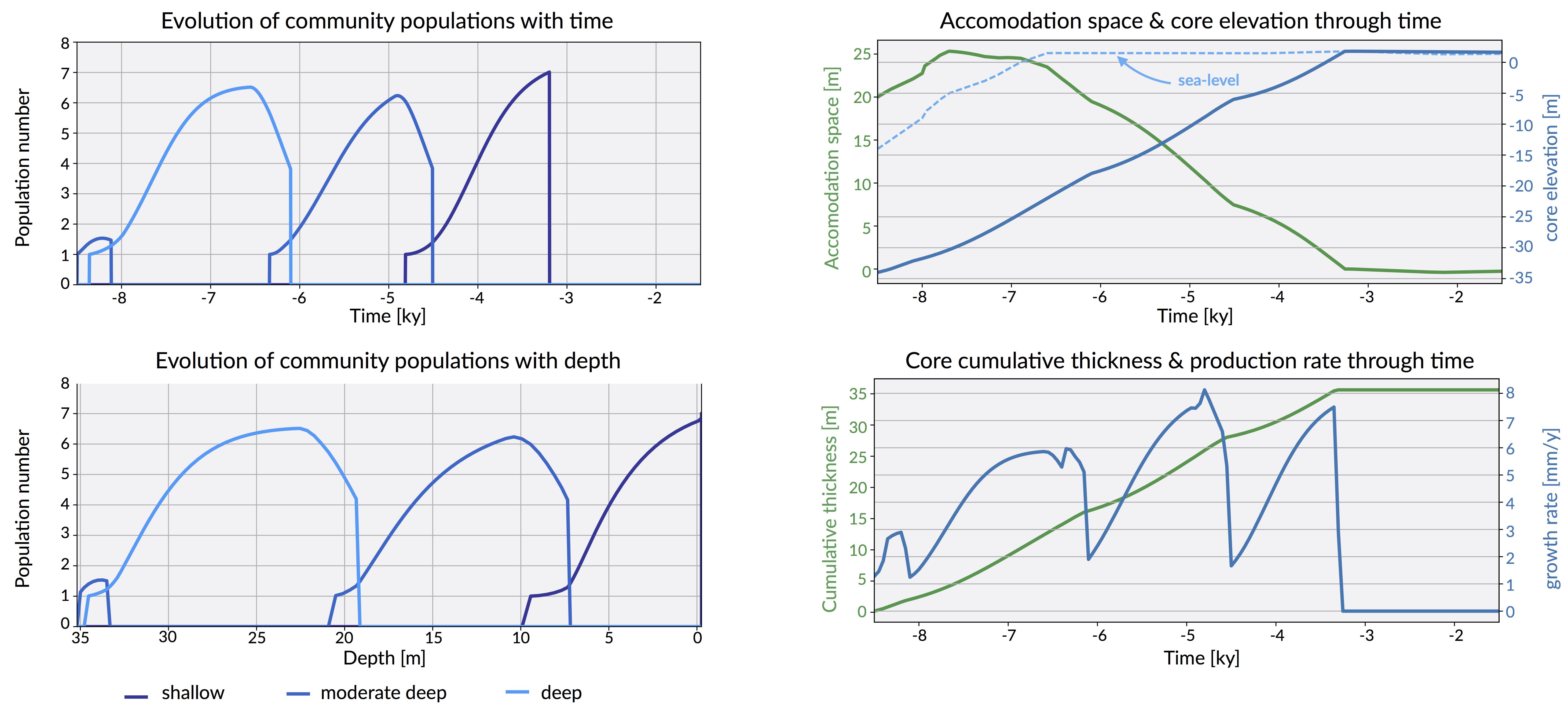
Change in community population over time and through depth associated to sea-level fluctuations imposed using Sloss et al. (2007) curve. As well as evolution of accommodation space, elevation, cumulative thickness and communities production rates simulated using pyReef-Core.

Schematic representation of synthetic data construction. (Left) Ideal shallowing-up fossil reef sequence representing a ‘catch-up’ growth strategy with associated assemblage compositions and changes, adapted from Dechnik (2016); (Right) Model output of synthetic core representing ideal shallowing-upward, ‘catch-up’ sequence.
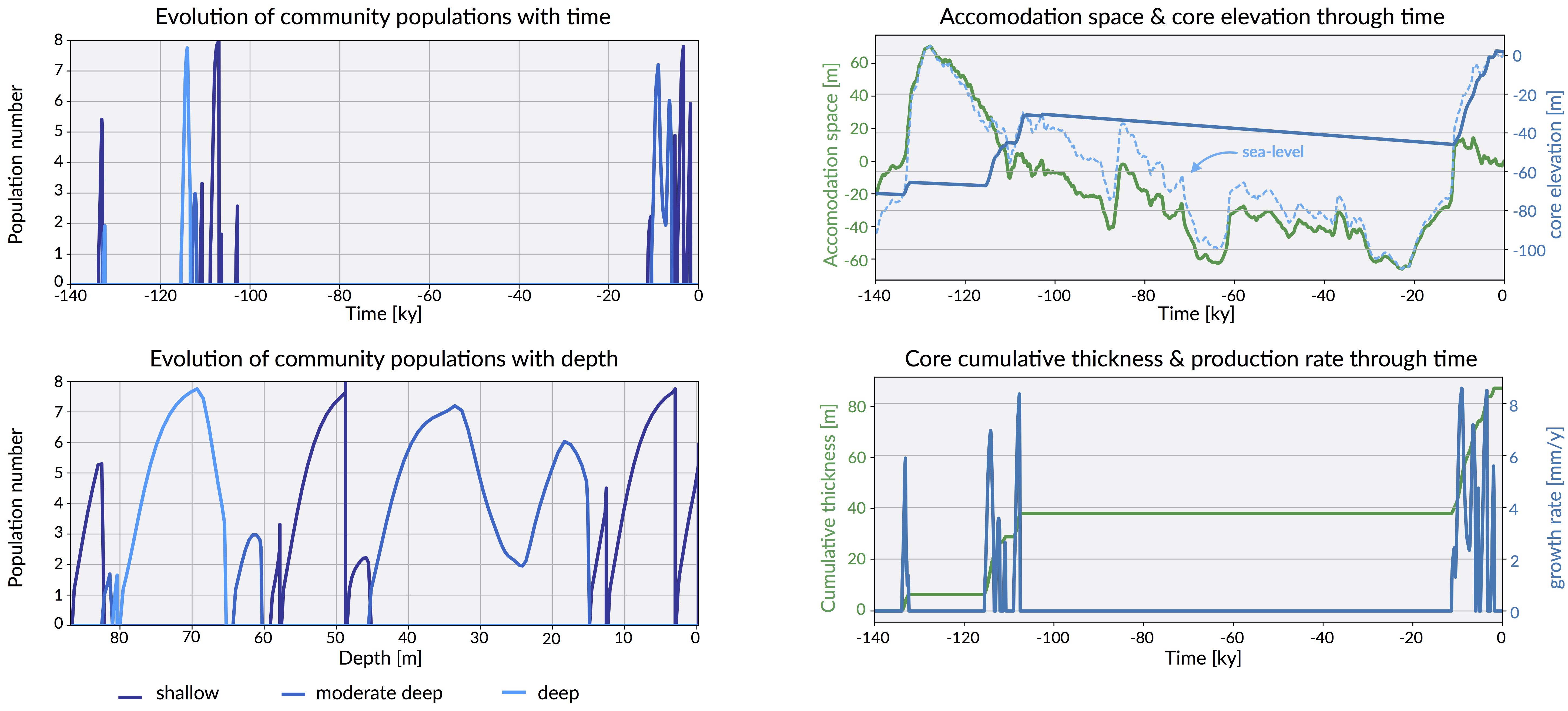
Change in community population over time and through depth associated to sea-level fluctuations imposed using Grant et al. (2012) curve. As well as evolution of accommodation space, elevation, cumulative thickness and communities production rates simulated using pyReef-Core.

Schematic representation of synthetic data construction.