R stuff for instagram vancouver 2016
See http://rolandtanglao.com/2017/09/08/p1-faceted-r-ggjoy-joyplot-with-colours-and-fill-colour/
colour_named_vector <-
setNames(as.character(average_colour_ig_van_jan2016$colourname),
         average_colour_ig_van_jan2016$colourname)
ggplot(average_colour_ig_van_jan2016,
  aes(x=hour, y= colourname , height=..density..))+
  geom_joy(scale=16, aes(colour=colour_named_vector)) +
  scale_colour_manual(values=colour_named_vector)
ggplot(average_colour_ig_van_jan2016, aes(x=hour, y= colourname , height=..density..))+
geom_joy(scale=16)
See http://rolandtanglao.com/2017/09/04/p2-remove-5-from-each-one-hour-period/
ggplot(gt5_h00_600colours, aes(x=colour))+
geom_density(mapping = aes(colour= colour_named_vector))+
scale_colour_manual(values=colour_named_vector)+
scale_y_continuous(limits = c(0,0.0012))+
theme_void()+theme(legend.position = 'none') +
theme(strip.background = element_blank(),strip.text.x = element_blank())
see http://rolandtanglao.com/2017/09/02/p2-0.0012version-is-better-density-plot-corrupted-for-art-copy/
II. Hex Colours + Greater than 5 occurences of colourname + truncate 0.002: Simple density plot for hour 0 i.e. midnight to 12:59a.m. with continuous colours from plotrix i.e. 600 colours
ggplot(gt5_h00_600colours, aes(x=colour))+
geom_density(mapping = aes(colour= colour_named_vector))+
scale_colour_manual(values=colour_named_vector)+
scale_y_continuous(limits = c(0,0.002))
I. Hex Colours + Greater than 5 occurences of colourname + truncate 0.005: Simple density plot for hour 0 i.e. midnight to 12:59a.m. with continuous colours from plotrix i.e. 600 colours
ggplot(gt5_h00_600colours, aes(x=colour))+
geom_density(mapping = aes(colour= colour_named_vector))+
scale_colour_manual(values=colour_named_vector)+
scale_y_continuous(limits = c(0,0.035))
Hex Colours + Greater than 5 occurences of colourname: Simple density plot for hour 0 i.e. midnight to 12:59a.m. with continuous colours from plotrix i.e. 600 colours
# use hex colours
colour_hex_strings_all = sapply(gt5_h00_600colours$sixhundred_colourint, function(x){
  function(x){
    sprintf(“#%6.6X”, x)})

colour_named_vector <- setNames(as.character(colour_hex_strings_all), colour_hex_strings_all)
ggplot(gt5_h00_600colours, aes(x=colour))+
geom_density(mapping = aes(colour= colour_named_vector))+
scale_colour_manual(values=colour_named_vector)
Greater than 5 occurences of colourname: Simple density plot for hour 0 i.e. midnight to 12:9a.m. with continuous colours from plotrix i.e. 600 colours
# let's remove <= 5
gt5_h00_600colours <- average_colour_ig_van_jan2016 %>%
filter(hour=="00") %>%
add_count(colourname) %>%
filter(n >5) %>%
rowwise() %>%
mutate(sixhundred_colourint = getnumericColour(colourname))

colour_named_vector <- setNames(as.character(gt5_h00_600colours$sixhundred_colourint), gt5_h00_600colours$sixhundred_colourint)

ggplot(gt5_h00_600colours, aes(x=colour))+
geom_density(mapping = aes(colour= colour_named_vector))+
scale_colour_manual(values=colour_named_vector)
Simple density plot for hour 0 i.e. midnight to 12:9a.m. with continuous colours from plotrix i.e. 600 colours
# use 600 values of 24 bit colour
library(tidyverse)
library(plotrix)

getnumericColour <-
  function(colorname) {
    colour_matrix=col2rgb(colorname)
    return(as.numeric(colour_matrix[1,1]) * 65536 +
             as.numeric(colour_matrix[2,1]) * 256 +
             as.numeric(colour_matrix[3,1]))
  }
csv_url =
"https://raw.githubusercontent.com/rtanglao/2016-r-rtgram/master/JANUARY2016/january2016-ig-van-avgcolour-id-mf-month-day-daynum-unixtime-hour-colourname.csv"
average_colour_ig_van_jan2016 = read_csv(csv_url)

h00_600colours <- average_colour_ig_van_jan2016 %>%
filter(hour=="00") %>%
rowwise() %>%
mutate(sixhundred_colourint = getnumericColour(colourname))

colour_named_vector <- setNames(as.character(h00_600colours$sixhundred_colourint), h00_600colours$sixhundred_colourint)

ggplot(h00_600colours, aes(x=colour))+
geom_density(mapping = aes(colour= colour_named_vector))+
scale_colour_manual(values=colour_named_vector)
- 1. simple plot for hour 0 (i.e. 00:00 to 00:59)
no00 <- singleton_colours_removed_average_colour_ig_van_jan2016_with_colourname %>%
filter(hour=="00") %>%
add_count(colourname) %>%
filter(nn != 1)
colour_named_vector <- setNames(no00$colourname, no00$colourname)
ggplot(no00, aes(x=colourname))+
  geom_density(mapping = aes(colour= colour_named_vector))+
  scale_colour_manual(values=colour_named_vector)
Output:

Remove singleton colournames and make a colour vector and plot them, need mapping in geom_density using colour vector and colour vector in scale_colour_manual and try a faceted plot
- 1. Remove singleton colournames
singleton_colours_removed_average_colour_ig_van_jan2016_with_colourname <-
average_colour_ig_van_jan2016_colourname %>%
add_count(colourname) %>%
filter(n != 1)
nrow(singleton_colours_removed_average_colour_ig_van_jan2016_with_colourname)
[1] 146463- 2. naive plot
ggplot(singleton_colours_removed_average_colour_ig_van_jan2016_with_colourname, aes(x=colourname))+
geom_density()
Result:
)%2Bgeom_density().png)
- 3. Make colour vector
# Don't need as.character() since it's already a character
colour_named_vector <- setNames
(singleton_colours_removed_average_colour_ig_van_jan2016_with_colourname$colourname, singleton_colours_removed_average_colour_ig_van_jan2016_with_colourname$colourname)- 4. Successful plot with graph "chrome"
ggplot(
singleton_colours_removed_average_colour_ig_van_jan2016_with_colourname,
aes(x=colourname))+
geom_density(mapping = aes(colour= colour_named_vector))+
scale_colour_manual(values=colour_named_vector)
Output:
)%2Bgeom_density(mapping%20%3D%20aes(colour%3D%20colour_named_vector))%2Bscale_colour_manual(values%3Dcolour_named_vector).png)
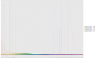
- 5. Successful plot without graph "chrome" i.e. theme_void() + remove legend
ggplot(
singleton_colours_removed_average_colour_ig_van_jan2016_with_colourname,
aes(x=colourname))+
geom_density(
mapping = aes(colour= colour_named_vector))+
scale_colour_manual(values=colour_named_vector)+
theme_void()+
theme(legend.position = 'none')+
theme(strip.background = element_blank(),strip.text.x = element_blank())
Output:
)%2Bgeom_density(mapping%20%3D%20aes(colour%3D%20colour_named_vector))%2Bscale_colour_manual(values%3Dcolour_named_vector)%20%2B%20theme_void().png)
Zazzle 2100 x 1800 output:

- 6. Faceted plot by hour
ggplot(
singleton_colours_removed_average_colour_ig_van_jan2016_with_colourname,
aes(x=colourname))+
geom_density(mapping = aes(
colour= colour_named_vector))+
scale_colour_manual(values=colour_named_vector)+
theme_void()+
theme(legend.position = 'none')+
theme(strip.background = element_blank(),strip.text.x = element_blank())+
facet_wrap(~ hour, nrow = 2)
Output:

- 1. AES maps but doesn't SET part 8888 :-) the colour instead it maps the variable, in this case colourname, to a set of levels and the levels are mapped to a default colour palette i.e. the plot shows up not in the colours of colourname but in the default colour palette! Code:
ggplot(average_colour_ig_van_jan2016_colourname,
aes(colourname, colour=colourname)) + geom_density()
And here's how it looks
Blogged here: http://rolandtanglao.com/2017/08/20/p1-naive-density-plot-instagram-vancouver-average-colour-january-2016/
- 1. After finally understanding density plots (thanks Kamyar!), I wrote this code
csv_url =
"https://raw.githubusercontent.com/rtanglao/2016-r-rtgram/master/JANUARY2016/january2016-ig-van-avgcolour-id-mf-month-day-daynum-unixtime-hour-colourname.csv"
average_colour_ig_van_jan2016_colourname = read_csv(csv_url)
ggplot(average_colour_ig_van_jan2016_colourname,
aes(colourname)) + geom_density()- 2. And here is the output (I used R Studio to make the output PNG 9740 x 6020 px) on flickr (on github: pdf, png):
- 1. Giving up on ggjoy for now :-)
- 2. Back to first principles of R and the tidyverse: http://rolandtanglao.com/2017/08/07/p1-mpg-scatterplot-average-colour-instagram-r-data-science/
- 3. Create January 1-31, 2016 instagram vancouver CSV with colournames, output file is: https://github.com/rtanglao/2016-r-rtgram/blob/master/JANUARY2016/january2016-ig-van-avgcolour-id-mf-month-day-daynum-unixtime-hour-colourname.csv:
cd JANUARY2016
Rscript ../part2-create-csv-ig-van-average-colour-jan2016.R- 4. Create part 3 naive scatterplot,
output file is:
part3-naive-january2016-ig-van-avgcolour-id-mf-month-day-daynum-unixtime-hour-colourname.png
Rscript ../part3-create-naive-scatterplot-colourname-hour.R- 5. Create part 4 with the dots of the scatterplot coloured like colourname i.e.
geom_pointuses the colour name literally (if you put the colour name inaesit will map the colour name to a level!) output file is:part4-colourname-aesthetic-january2016-ig-van-avgcolour-id-mf-month-day-daynum-unixtime-hour-colourname.png
Rscript ../part4-create-colourname-with-colourname-aesthetic-scatterplot-hour.RHere's the part 4 output:

Rscript ../average-colour-by-hour-ggjoy-from-csv.R 31-january2016-ig-van-avgcolour-id-mf-month-day-daynum-unixtime-hour.csv
Error in FUN(X[[i]], ...) : need at least 2 data points
Calls: main ... <Anonymous> -> f -> <Anonymous> -> f -> vapply -> FUN
Execution halted- 2.But I have two data points! namely for example the first 6 rows I have 3 rows with
indianred4
 colour                             id dayofweek.month.dayofmonth daynumber   unixtime  hour colourname
    <chr>                          <chr>                      <chr>     <int>      <int> <int>      <chr>
1 #546363 1174465369140103047_2176611536                   SunJan31        31 1454227203     0     gray37
2 #ACA8A8 1174465451560169285_2137478482                   SunJan31        31 1454227213     0   darkgray
3 #6B3434 1174465462824925338_2250967365                   SunJan31        31 1454227215     0 indianred4
4 #4B3E3E  1174465565628114803_177763144                   SunJan31        31 1454227227     0     gray26
5 #803A3A  1174465617924150379_361059564                   SunJan31        31 1454227233     0 indianred4
6 #704141 1174465676122308807_1537167607                   SunJan31        31 1454227240     0 indianred4
cd /Users/rtanglao/Dropbox/GIT/2016-r-rtgram/JANUARY2016/24SQUARES-PER-DAYparallel Rscript ../../twenty-four-square-pie-chart-from-csv.R '{}' ::: ../??-january2016-ig-van-avgcolour-id-mf-month-day-daynum-unixtime-hour.csvmkdir TRIMMEDparallel convert -trim '{}' 'TRIMMED/{}' ::: *.pngcd TRIMMEDls -1 *.png >31pngs.txtgm montage -verbose -adjoin -tile 7x6 +frame +shadow +label -adjoin -geometry '1023x684+0+0<' null: null: null: null: null: @31pngs.txt null: null: null: null: null: null: ig-van-2016-one-top-colour-square-per-hour-01-31january2016-square-piechart.png
Put the january 1-31, 2016 github dataset up on octopub (which is on github!)
- for each day.csv
- loop over all 24 hours (do i really need a loop? probably not)
- get that hour's subset from the CSV file, average the subset, add the average to that hour's dataframe
- add colourname to the hour's dataframe and the graph the hour's dataframe
- What shall I do next besides the pull request for waffle and/or the github issue?:
- Maybe average colour over each day and then do a June 1-May 27, 2016 graphic?
- Maybe train a neural network with the likes (weight 0.5), comments (weight 1.0) with my instagram photos from 2014-2016?
cd /Users/rtanglao/Dropbox/GIT/2016-r-rtgram/JANUARY2016/FIXED-WAFFLE-3000parallel Rscript ../../file-numphotos-square-piechart.R '{}' 3000 ::: ../*-january2016-ig-van-avgcolour-id-mf-month-day-daynum-unixtime-hour.csvmkdir TRIMMEDparallel convert -trim '{}' 'TRIMMED/{}' ::: 3000*.pngcd TRIMMEDls -1 3000*.png >31pngs.txtgm montage -verbose -adjoin -tile 7x6 +frame +shadow +label -adjoin -geometry '1023x308+0+0<' null: null: null: null: null: @31pngs.txt null: null: null: null: null: null: ig-van-2016-top3000-topcolour-sorted-3000-squares-01-31january2016-square-piechart.png
The solution which I still haven't tested:
From stack overflow repeating vector of letters:
letters658 = make.unique(rep(letters, length.out = 658), sep='') #use letters658 instead of LETTERS R constantThe above code makes up for the R constant LETTERS only having 26 levels when R has 657 colours (add 1 since
waffle() starts at 'B' instead of 'A'). So having 657 letters will allow all R colours to be plotted safely instead of any colour beyond the
first 26 being turned into 'not a number' i.e. NA.
pseudo code: pass in number of squares as a command line argument, do (2500-1000)/2 + 1000 i.e. a binary search for where it breaks startg with 1750
Algorithm: take 1st 2500 photos, get colournames, sort by descending frequency of colournames and then take the first 1000 photos to form a square pie chart graph of <=1000 squares
/Users/rtanglao/Dropbox/GIT/2016-r-rtgram/JANUARY2016/CUMULATIVE-SUM-1000mkdir TRIMMEDls -1 ../*-january2016-ig-van-avgcolour-id-mf-month-day-daynum-unixtime-hour.csv | xargs -n 1 Rscript ../../cumulativesum-size0.1-first2500-void-square-piechart-from-csv.Rparallel convert -trim '{}' 'TRIMMED/{}' ::: cumulative-sum*.png# results in 750x480 and 768x480 pngcd TRIMMED; ls -1 >31pngs.txtgm montage -verbose -adjoin -tile 7x6 +frame +shadow +label -adjoin -geometry '768x480+0+0<' null: null: null: null: null: @31pngs.txt null: null: null: null: null: null: ig-van-2016-top2500-topcolour-sorted-1000-squares-01-31january2016-square-piechart.pnggm montage -verbose -adjoin -tile 7x6 +frame +shadow +label -adjoin -geometry '750x480+0+0<' null: null: null: null: null: @31pngs.txt null: null: null: null: null: null: 750-ig-van-2016-top2500-topcolour-sorted-1000-squares-01-31january2016-square-piechart.png<script async src="//embedr.flickr.com/assets/client-code.js" charset="utf-8"></script>

cd /Users/rtanglao/Dropbox/GIT/2016-r-rtgram/JANUARY2016/DIV5-SIZE0.1mkdir TRIMMEDls -1 ../*-january2016-ig-van-avgcolour-id-mf-month-day-daynum-unixtime-hour.csv | xargs -n 1 Rscript ../../div5-size0.1-first2500-void-square-piechart-from-csv.Rparallel convert -trim '{}' 'TRIMMED/{}' ::: first2500-div5-size0.1-*.png
cd /Users/rtanglao/Dropbox/GIT/2016-r-rtgram/JANUARY2016/DIV10-SIZE0.1ls -1 ../*-january2016-ig-van-avgcolour-id-mf-month-day-daynum-unixtime-hour.csv | xargs -n 1 Rscript ../../div10-size0.1-first2500-void-dquare-piechart-from-csv.Rmkdir TRIMMEDparallel convert -trim '{}' 'TRIMMED/{}' ::: first2500-div10-size0.1-square-piechart-colourname-*.png
cd /Users/rtanglao/Dropbox/GIT/2016-r-rtgram/JANUARY2016/SIZE0.1ls -1 ../*-january2016-ig-van-avgcolour-id-mf-month-day-daynum-unixtime-hour.csv | xargs -n 1 Rscript ../../size0.1.-first2500-void-square-piechart-from-csv.Rmkdir TRIMMEDparallel convert -trim '{}' 'TRIMMED/{}' ::: first2500-size0*.png
- use cumsum to compute a cumulative sum column ``sept01countcolourname$numphotos <- cumsum(sept01countcolourname$freq)```
- then use head with a conditional on the cumulative sum get first 2000
subset(sept01countcolourname, sept01countcolourname$numphotos <2001)
- fixed bug changed 2501 to 2500!
cd /Users/rtanglao/Dropbox/GIT/2016-r-rtgram/JANUARY2016- ``````ls -1 *-january2016-ig-van-avgcolour-id-mf-month-day-daynum-unixtime-hour.csv | xargs -n 1 Rscript ../first2500-colourname-void-square-piechart-from-csv.R```
parallel convert -trim '{}' 'FIRST2500-TRIMMED/{}' ::: first2500*.png
Rscript first6-ig-van-01january2016-square-piechart.R
output:<script async src="//embedr.flickr.com/assets/client-code.js" charset="utf-8"></script>
cd /Users/rtanglao/Dropbox/GIT/2016-r-rtgram/JANUARY2016ls -1 *-january2016-ig-van-avgcolour-id-mf-month-day-daynum-unixtime-hour.csv | xargs -n 1 Rscript ../first2500-colourname-void-square-piechart-from-csv.R- trim off white space:
mkdir FIRST2500-TRIMMED parallel convert -trim '{}' 'FIRST2500-TRIMMED/{}' ::: first2500*.pngcitation: O. Tange (2011): GNU Parallel - The Command-Line Power Tool, ;login: The USENIX Magazine, February 2011:42-47. actually the above is wrong because convert -trim truncates white columns, ok then we should use 1026x475px not trim
cd /Users/rtanglao/Dropbox/GIT/2016-r-rtgram/JANUARY2016../faceted-by-daynumber-colourname-void-square-piechart-from-csv.R january2016-ig-van-avgcolour-id-mf-month-day-daynum-unixtime-hour.csv- Use iron() to display all 31? Because it doesn't work, maybe because faceting isn't supported?:
Error in layout_base(data, vars, drop = drop) : At least one layer must contain all variables used for facetting
cd /Users/rtanglao/Dropbox/GIT/2016-r-rtgram/JANUARY2016ls -1 *-january2016-ig-van-avgcolour-id-mf-month-day-daynum-unixtime-hour.csv | xargs -n 1 Rscript ../colourname-void-square-piechart-from-csv.R
Rscript first3-ig-van-01january2016-square-piechart.R# theme_void doesn't work, gives us 1 colour only!open 1st3-ig-van-01january-2016-squarepiechart.pngoutput:<script async src="//embedr.flickr.com/assets/client-code.js" charset="utf-8"></script>

mkdir JANUARY 2016; cd !$; cp ../january2016-ig-van-avgcolour-id-mf-month-day-daynum-unixtime-hour.csv .../splitCSVForAMonthInto31CSFfiles.rb january2016-ig-van-avgcolour-id-mf-month-day-daynum-unixtime-hour.csvls -1 *-january2016-ig-van-avgcolour-id-mf-month-day-daynum-unixtime-hour.csv | xargs -n 1 Rscript ../colourname-void-piechart-from-csv.Rls -1 *.png > 31pngs.txtgm montage -verbose -adjoin -tile 7x6 +frame +shadow +label -adjoin -geometry '1920x1920+0+0<' null: null: null: null: null: @31pngs.txt null: null: null: null: null: null: 01-31january2016-piechart.png# Week starts on a Sunday and January 1 is a Friday so add 5 nulls at the beginning, January 31 is a Sunday so add 6 nulls at the endgm convert 01-31january2016-piechart.png 01-31january2016-piechart.jpg# And post jpeg to flickr :-)

How to make a named character vector in R - useful if we ever want have a legend with colours in a pie chart.
- hourly failed but i got it working!
Rscript scale-color-manual-first3-ig-van01january2016-piechart.Rmore info: http://rolandtanglao.com/2016/07/31/p3-simplest-ggplot2-pie-chart-with-colors-as-bar-values-and-a-legend/
- let's try hourly
Rscript ig-van-01january2016-piechart.R - output: ig-van-01january-2016-barchart.png
today let's try theme_void() - it's great! removed all chrome!
Rscript ig-van-january2016-piechart-as-barchart.R# output ig-van-january-2016-piechart-as-barchart.pngmv ig-van-january-2016-barchart.png theme-void-ig-van-january-2016-barchart.png
 small multiples vancouver 2016 january piechart")
Rscript ig-van-january2016-piechart-as-barchart.R# output ig-van-january-2016-piechart-as-barchart.pngRscript ig-van-january2016-piechart.R#output ig-van-january-2016-barchart.png There's a BUG in layout of small multiples hmmm lots of bugs? is there a bug in my script or in my data that causes the large white slices in the following output png:

)%2Bgeom_density().png)