DNET - Distribution Network Evaluation Tool

• Features
• Overview
• Installing
• Network data
• Tutorial
• Additional notes
• References

Features

• Highly efficient analysis tool for power distribution networks
• Power loss minimization (nonconvex optimization over several hundreds of variables!)
• Distribution network verification to guarantee secure restoration
• Featuring Graphillion, an efficient graphset operation library
• Open source MIT license
• Additional benefits from Python: fast prototyping, easy to teach, and multi-platform

Overview

DNET (Distribution Network Evaluation Tool) is an analysis tool that works with power distribution networks for efficient and stable operation such as loss minimization and verification.

Power distribution networks consist of several switches. The structure, or configuration, can be reconfigured by changing the open/closed status of the switches depending on the operational requirements. However, networks of practical size have hundreds of switches, which makes network analysis a quite tough problem due to the huge size of search space. Moreover, power distribution networks are generally operated in a radial structure under the complicated operational constraints such as line capacity and voltage profiles. The loss minimization and verification in a distribution network is a hard nonconvex optimization problem.

DNET finds the best configuration you want with a great efficiency. All feasible configurations are examined without stuck in local minima. DNET handles complicated electrical constraints with realistic unbalanced three-phase loads. We've optimized and verified a large distribution network with 468 switches using DNET; please see papers listed in references in detail. We believe that DNET takes you to the next stage of power distribution network analysis.

DNET can be used freely under the MIT license. It is mainly developed by JST ERATO Minato project. We would really appreciate if you would refer to our paper and address our contribution on the use of DNET in your paper.

Takeru Inoue, Keiji Takano, Takayuki Watanabe, Jun Kawahara, Ryo Yoshinaka, Akihiro Kishimoto, Koji Tsuda, Shin-ichi Minato, and Yasuhiro Hayashi, "Distribution Loss Minimization with Guaranteed Error Bound," IEEE Transactions on Smart Grid, vol.5, issue.1, pp.102-111, January 2014. (pdf)

Takeru Inoue, Norihito Yasuda, Shunsuke Kawano, Yuji Takenobu, Shin-ichi Minato, and Yasuhiro Hayashi, "Distribution Network Verification for Secure Restoration by Enumerating All Critical Failures," IEEE Transactions on Smart Grid, October 2014. (pdf)

DNET is still under the development. The current version supports power loss minimization, configuration search, and verification. We are thinking of service restoration for future releases.

We really appreciate any pull request and patch if you add some changes that benefit a wide variety of people.

Installing

Requirements

Python

To use DNET, you need Python version 2.7 or Python 3.4.

Quick install

Just type:

$ sudo pip install pydnet  # not "dnet", but "pydnet"

and an attempt will be made to find and install an appropriate version that matches your operating system and Python version.

All the required modules should be automatically installed along with DNET; if not, please install them by manual, as follows:

$ sudo pip install graphillion
$ sudo pip install networkx
$ sudo pip install pyyaml

Graphillion and NetworkX are Python modules for graphs, while PyYAML is another Python module for a compact syntax called YAML.

Installing from source

You can install from source by downloading a source archive file (tar.gz or zip) or by checking out the source files from the GitHub source code repository.

Source archive file

1. Download the source (tar.gz or zip file) from https://github.com/takemaru/dnet
2. Unpack and change directory to the source directory (it should have the file setup.py)
3. Run python setup.py build to build
4. (optional) Run python setup.py test -q to execute the tests
5. Run sudo python setup.py install to install

GitHub repository

1. Clone the Dnet repository git clone https://github.com/takemaru/dnet.git
2. Change directory to "dnet"
3. Run python setup.py build to build
4. (optional) Run python setup.py test -q to execute the tests
5. Run sudo python setup.py install to install

If you don't have permission to install software on your system, you can install into another directory using the -user, -prefix, or -home flags to setup.py. For example:

$ python setup.py install --prefix=/home/username/python
  or
$ python setup.py install --home=~
  or
$ python setup.py install --user

If you didn't install in the standard Python site-packages directory you will need to set your PYTHONPATH variable to the alternate location. See http://docs.python.org/inst/search-path.html for further details.

Network data

DNET requires network data, which includes network topology (line connectivity and switch positions), loads, and impedance. The data must be formatted by YAML syntax. We explain the formatting rules using an example, data/test.yaml in the DNET package. This example network consists of three feeders and 16 switches, as shown in the figure.

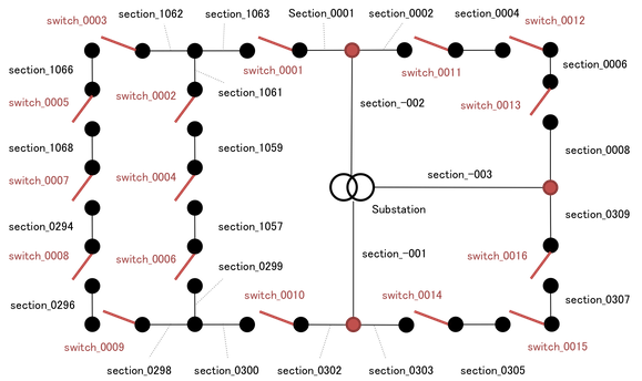
The data file is divided into three parts; nodes, sections, and switches. Since YAML rules are quite simple, we believe it is not so difficult to understand it.

Nodes

The "nodes" part describes nodes, at which a switch and/or section(s) are connected. In the above example network, nodes are indicated by black or red circles. The following YAML data shows some nodes in the example network; three sections are connected at the first node (i.e., section_-001, section_0302, and section_0303), while a section and a switch is connected at the fourth node (i.e., section_0302 and switch_0010).

nodes:
- [section_-001, section_0302, section_0303]
- [section_-002, section_0001, section_0002]
- [section_-003, section_0008, section_0309]
- [section_0302, switch_0010]
:

Sections

The "sections" part describes section information including load and impedance. In DNET, loads are assumed to be unbalanced three-phase and be connected in delta. Loads are also assumed to be uniformly distributed along a line section, and are modeled as constant current, not as power (see Section 2 in theory.pdf for more detail).

In the data file, load and impedance are specified by six values, which are real and imaginary parts of the three phases; for section_-001 in the following YAML, load current is 16.3225894 + 0j in the 0-th phase, and impedance is 0.0684 + 0.3678805j in the all phases. Substation attribute indicates whether the line section is directly connected to a feeding point in the substation.

sections:
  section_-001:
    impedance: [0.0864, 0.3678805, 0.0864, 0.3678805, 0.0864, 0.3678805]
    load: [16.3225894, 0, 16.3225894, 0, 1.29105e-11, 0]
    substation: true
:

Switches

The "switches" part specifies the switch order in a list. We have to be careful to assign the order. Switches should be ordered based on the proximity in the network as shown in the figure, because DNET's efficiency highly depends on the order. For the loss minimization, switches must be ordered so as not to step over junctions connected to a substation as few as possible (such junctions are indicated by red circles in the figure); see Sections 4.1 and 5.1 in theory.pdf for more detail.

switches:
- switch_0001
- switch_0002
- switch_0003
:

Fukui-TEPCO format

Network data in the Fukui-TEPCO format can be also accepted in DNET. Since Fukui-TEPCO format lacks switch indicators, you have to add file sw_list.dat that includes switch names; see examples in data/test-fukui-tepco/ in detail.

Tutorial

We assume network data used in this tutorial is stored in a directory data/. Download file data/test.yaml or all files in data/test-fukui-tepco/ and put it into the directory before beginning the tutorial.

Start the Python interpreter and import DNET.

$ python
>>> from dnet import Network

You might need to change the maximum current and voltage range for your own data. The default values are given as follows.

>>> from math import sqrt
>>> Network.MAX_CURRENT     = 300
>>> Network.SENDING_VOLTAGE = 6600 / sqrt(3)
>>> Network.VOLTAGE_RANGE   = (6300 / sqrt(3), 6900 / sqrt(3))

Load the network data as follows.

>>> nw = Network('data/test.yaml')

If your data is in the Fukui-TEPCO format, specify data directory with the format type (this is just for the explanation, don't do this line for this tutorial).

>>> nw = Network('data/test-fukui-tepco', format='fukui-tepco')

We can access to the loaded network data (if you've loaded the Fukui-TEPCO format data, the switch numbers are different).

>>> nw.nodes
[['section_-001', 'section_0302', 'section_0303'], ['section_-002', 'section_0001', 'section_0002'], ['section_-003', 'section_0008', 'section_0309'], ['section_0302', 'switch_0010'], ['section_0300', 'switch_0010'], ...
>>> nw.sections
{'section_1068': {'load': [(23.87780659+4.33926456j), (23.1904931+4.214360495j), (2.2606e-12+4.10814e-13j)], 'impedance': [(0.1539+0.4512584j), (0.1539+0.4512584j), (0.1539+0.4512584j)], 'substation': False}, ...
>>> nw.switches
['switch_0001', 'switch_0002', 'switch_0003', 'switch_0004', 'switch_0005', 'switch_0006', 'switch_0007', 'switch_0008', 'switch_0009', 'switch_0010', 'switch_0011', 'switch_0012', 'switch_0013', 'switch_0014', 'switch_0015', 'switch_0016']

Then, enumerate all feasible configurations as follows.

>>> configs = nw.enumerate()  # all feasible configurations

Object configs is an instance of class ConfigSet, which supports similar interface with graphillion.GraphSet (a configuration can be regarded as a forest of graph). We can utilize the rich functions provided by Graphillion, such as counting, search, and iteration for configurations in the object.

Count the number of all the feasible configurations.

>>> configs.len()
111L

This shows that the network has 111 feasible configurations.

Search for configurations by a query; e.g., switch 2 is closed while switch 3 is open, but statuses of the other switches are not cared.

>>> configs_w2_wo3 = configs.including('switch_0002').excluding('switch_0003')
>>> configs_w2_wo3.len()
15L

These configurations can be visited one by one using an iterator as follows.

>>> for config in configs_w2_wo3:
...     config
...
['switch_0001', 'switch_0011', 'switch_0002', 'switch_0005', 'switch_0004', 'switch_0007', 'switch_0008', 'switch_0009', 'switch_0010', 'switch_0014', 'switch_0012', 'switch_0015']
['switch_0001', 'switch_0011', 'switch_0002', 'switch_0005', 'switch_0004', 'switch_0007', 'switch_0008', 'switch_0009', 'switch_0010', 'switch_0014', 'switch_0012', 'switch_0016']
['switch_0001', 'switch_0011', 'switch_0002', 'switch_0005', 'switch_0004', 'switch_0007', 'switch_0008', 'switch_0009', 'switch_0010', 'switch_0012', 'switch_0016', 'switch_0015']
:

Each line shows a configuration, which is represented by a set of closed switches.

We select 5 configurations uniformly randomly with a random iterator returned by rand_iter(), and calculate the average loss over them (i.e., random sampling).

>>> i = 1
>>> sum = 0.0
>>> for config in configs_w2_wo3.rand_iter():
...     sum += nw.loss(config)
...     if i == 5:
...         break
...     i += 1
...
>>> sum / 5
85848.080193479094

We search for the minimum loss configuration from all feasible configurations enumerated above.

>>> optimal_config = nw.optimize(configs)
>>> optimal_config  # closed switches in the optimal configuration
['switch_0001', 'switch_0002', 'switch_0003', 'switch_0005', 'switch_0006', 'switch_0008', 'switch_0009', 'switch_0010', 'switch_0011', 'switch_0013', 'switch_0014', 'switch_0016']

We can obtain switches that are open in the optimal configuration, by subtracting all the switches from the closed switches.

>>> set(nw.switches) - set(optimal_config)
set(['switch_0004', 'switch_0007', 'switch_0012', 'switch_0015'])

The loss value at the optimal configuration is calculated as follows.

>>> nw.loss(optimal_config, is_optimal=True)
(72055.704210858064, 69238.43315354317)

With is_optimal option, loss() returns the loss at the optimal configuration as well as the lower bound, which means a theoretical bound under which loss never be (see Section 3.3 in theory.pdf in detail). In this example, the minimum loss is 69734 while the lower bound is 67029.

Finally, we enumerate all the line cuts, under which the distribution network cannot be restored. The following enumerate such "unrestorable cuts" with size of two or less.

>>> unrestorable_cuts = nw.unrestorable_cuts(2)
>>> len(unrestorable_cuts)
25
>>> unrestorable_cuts[0]
(('section_0299', 'section_0298', 'section_0300'), ('section_0006',)))

This network has 25 unrestorable cuts with size of two or less. One of them includes a cut either of section 299, 298, or 300, and another cut of section 6. If the two cuts are placed at the same time, the network is still physically connected but cannot be restored due to the violation of electrical constraints.

In this tutorial, we examined small network with 16 switches. DNET, however, can work with a much larger network with hundreds of switches, as demostrated in our papers in references.

Additional notes

• DNET has been modified from our paper's version. The current version is much faster than the paper version. Some loss values presented in the paper are inconsistent with those by the current version since implementation bugs have been fixed, though they have no impact on conclusions of the paper.

• DNET assumes that just switches are controllable in a distribution network while other components like capacitors are ignored; we consider the distribution network analysis as a combinatorial problem, in which the variable is open/closed status of the switches.

• In DNET, section loads must be given as constant current. Line current is calculated by sweeping backward to sum up downstream section loads. This is because our loss minimization method depends on this backward sweeping; see Section 3.1 in theory.pdf in detail. However, if you are interested in only the configuration search, line current can be calculated in another way with section loads of constant power; fix _calc_current() and _satisfies_electric_constraints() in dnet/network.py.

• DNET assumes that all section loads are non-negative. This can be an issue if introducing distributed generators; see Sections 4.1 and 8 in theory.pdf for more detail.

• DNET can select configurations feasible for multiple load profiles by the intersection operation provided by Graphillion. You must use the same network topology and the same switch order for all load profiles.

>>> day_nw   = Network('data/day.yaml')
>>> night_nw = Network('data/night.yaml')
>>> day_configs   = day_nw.enumerate()    # feasible configurations just for day load profile
>>> night_configs = night_nw.enumerate()  # feasible configurations just for night load profile
>>> day_and_night_configs = day_configs & night_configs  # feasible for both profiles

• In the loss minimization, switches between a substation and a junction are assumed to be closed. This is because such junctions (i.e., red circles in the figure) must be energized in any configurations in our loss minimization method; see Section 4.1 in theory.pdf for more detail.

• The search space used in the optimization process is a directed acyclic graph. The shortest path on the graph indicates the optimal solution, and the path weight corresponds to the minimum loss. We can retrieve the graph with their weights and configuration (vertex numbers in the following example may be different in your environment). The starting and ending vertices are also shown.

>>> optimal_config = nw.optimize(configs)
>>> graph = nw.search_space.graph
>>> for u, v in graph.edges():
...     u, v, graph[u][v]['weight'], graph[u][v]['config']  # an edge with its weight and config
...
('4082', 'T', 236.19071155693283, set(['switch_0016', 'switch_0014']))
('38', 'T', 236.19071155693283, set(['switch_0016', 'switch_0014']))
('46', '38', 196.46357613253261, set(['switch_0013', 'switch_0012']))
:
>>> nw.search_space.start, nw.search_space.end  # starting and ending vertices
('4114', 'T')

References

• Yuji Takenobu, Norihito Yasuda, Shunsuke Kawano, Yasuhiro Hayashi, and Shin-ichi Minato, "Evaluation of Annual Energy Loss Reduction Based on Reconfiguration Scheduling," IEEE Transactions on Smart Grid, September 2016. (doi)
• Y. Takenobu, S. Kawano, Y. Hayashi, N. Yasuda and S. Minato, "Maximizing hosting capacity of distributed generation by network reconfiguration in distribution system," Proc. of Power Systems Computation Conference (PSCC), pp.1-7, June 2016. (doi)
• Takeru Inoue, Norihito Yasuda, Shunsuke Kawano, Yuji Takenobu, Shin-ichi Minato, and Yasuhiro Hayashi, "Distribution Network Verification for Secure Restoration by Enumerating All Critical Failures," IEEE Transactions on Smart Grid, October 2014. (doi)
• Takeru Inoue, Keiji Takano, Takayuki Watanabe, Jun Kawahara, Ryo Yoshinaka, Akihiro Kishimoto, Koji Tsuda, Shin-ichi Minato, and Yasuhiro Hayashi, "Distribution Loss Minimization with Guaranteed Error Bound," IEEE Transactions on Smart Grid, vol.5, issue.1, pp.102-111, January 2014. (pdf)
• Takeru Inoue, "Theory of Distribution Network Evaluation Tool." theory.pdf
• Graphillion - Fast, lightweight graphset operation library