PsyCalibrator: an open-source package for display gamma calibration and luminance and color measurement
Zhicheng Lin1, Qi Ma2, Yang Zhang2
1 School of Humanities and Social Science, The Chinese University of Hong Kong, Shenzhen, China 518172
2 Department of Psychology, Soochow University, Suzhou, Jiangsu, China 215000
This is the step-by-step photometer tutorial portion of the article. The tutorial includes the following seven steps. For luminance/color measurement, follow Steps 1 to 4; for monitor correction (linearization), follow all the steps except Step 4.
- Step 1: Obtain required instrument and software
- Step 2: Install Spyder driver
- Step 3: Make “PsyCalibrator” accessible to MATLAB
- Step 4: Luminance and color measurement
- Step 5: Calibration measurement
- Step 6: Data fitting
- Step 7: Apply or remove gamma correction
- Reference
-
Instrument:
Spyder5orSpyderXNote:
SpyderXis the newer model. For bothSpyder5andSpyderX, there are different versions available, but the only difference between the different versions (e.g., Express, Pro, and Elite) is the accompanying software package provided by Spyder. Since our calibration method does not use this provided software but only the hardware, any version of Spyder will work. -
A computer with the following software:
- MATLAB (common commercial software) or GNU Octave (a free alternative to MATLAB; for simplicity, below we will refer to MATLAB only) and Psychtoolbox.
- Psychtoolbox (free software available at http://psychtoolbox.org)
- PsyCalibrator (free at: https://github.com/yangzhangpsy/PsyCalibrator)
Note: The software package includes both original files provided by the authors as well as files written by others (specifically, the file “spyderDriverWin” is extracted from Argyll V2.1.2, available at http://www.argyllcms.com; the file “makeCLUT_APL” is modified from Mcalibrator2, available at https://github.com/hiroshiban/Mcalibrator2)
🔴🔴🔴**a) If you are using the SpyderX hardware and versions of Psychtoolbox equal to or after 3.0.19 (note that the "Virtuality" update was released on February 17th, 2023), or b) if the returned information by running PsychHID in MATLAB, contains the following content([countOrRecData] = PsychHID('USBBulkTransfer', usbHandle, endPoint, length [, outData][, timeOutMSecs=10000])), You can proceed directly to Step 3. This is because the new versions of Psychtoolbox come with an added USBbulktransfer function, which enables us to support the use of the built-in drivers in Windows 10/11 for controlling the SpyderX hardware.**🔴🔴🔴
If you are using Linux or Mac, there is no need to install the driver for the photometer. But if you are using Windows, you need to install the driver for the photometer. To check whether the driver is already installed, insert the device (e.g., Spyder5) into a USB port on the computer. Then open the "Device Manager" menu in Windows Settings (you can search "Device Manager" in the search bar at the bottom left of the desktop). If the driver has already been installed, you should see a USB icon showing “Spyder5 (Argyll)”, as highlighted in the red rectangle in Figure 1.
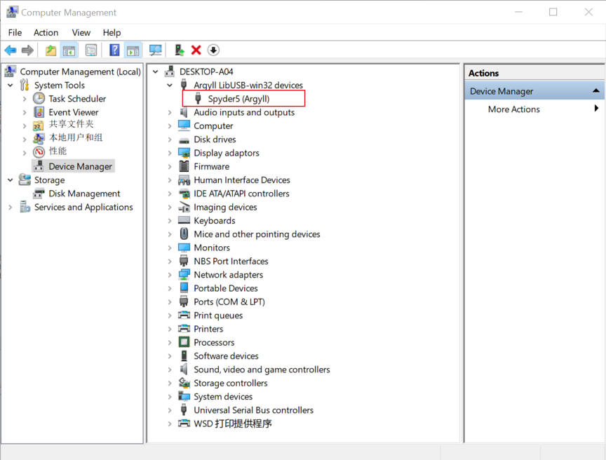
Figure 1. Device Manager showing Spyder5 with the driver installed.
On the other hand, if the driver has not been installed, then you may see an exclamation mark (!) appearing before the device name, as highlighted in the red rectangle in Figure 2 (note that if you have installed the software that comes with Spyder, you will not see the exclamation mark). Or you may simply see the device under “Universal Serial Bus devices” (bottom, Figure 2). In either case, we need to install the calibration driver as offered in the “PsyCalibrator” package, by following the steps below.
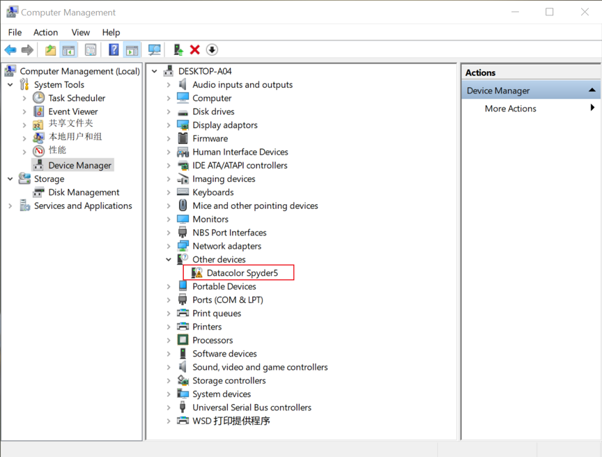
Figure 2. Device Manager showing the Spyder device with the driver not installed.
2.1. First, right-click on the device name “Datacolor Spyder5” (or “Datacolor SpyderX”), which should open up a menu as in Figure 3. Click "Update driver".
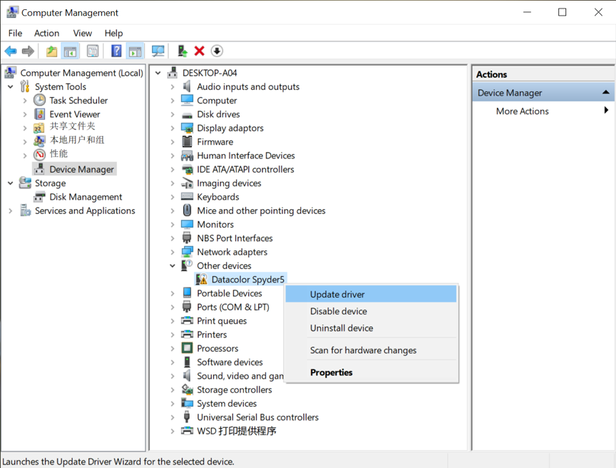
Figure 3. Update driver for the photometer.
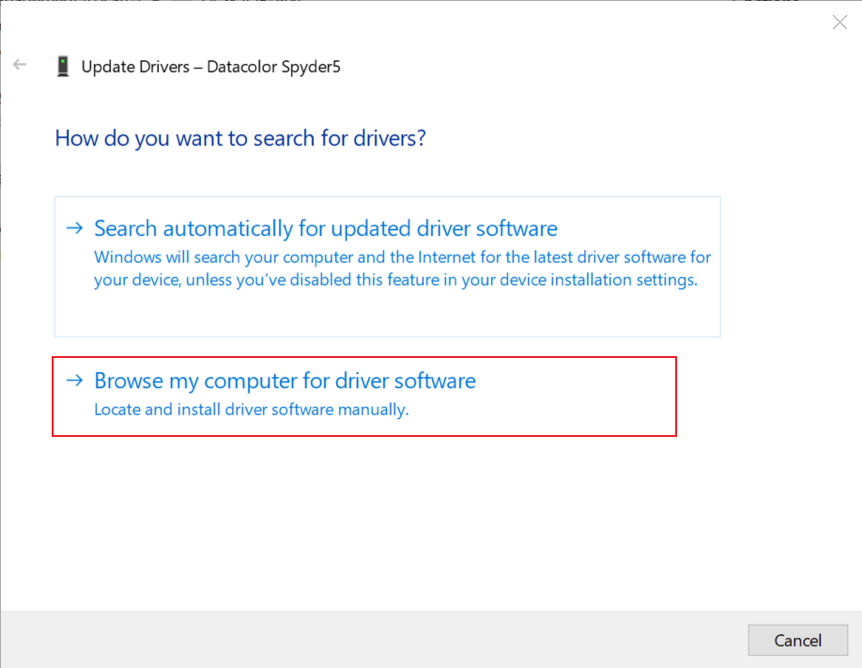
2.2. Then, select "Browse my computer for driver software" (Figure 4).
Figure 4. Options for installing the driver.
2.3. Click "Browse" to find the driver software ("spyderDriverWin") in the "PsyCalibrator" folder, and then click "Next" (Figure 5 top). If you see “The best drivers for your device are already installed” (Figure 5 bottom), then instead of the “Browse” option above, you need to use the option “Let me pick from a list of available drivers on my computer” (then choose “Hard Disk…”, then “Browse” to find the same driver folder, then “OK”, and “Next”).
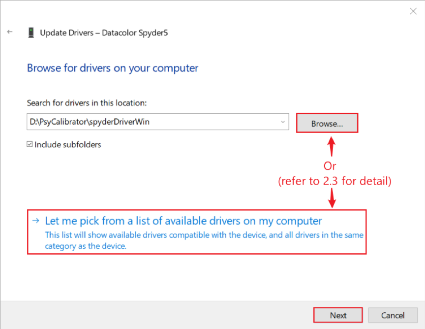
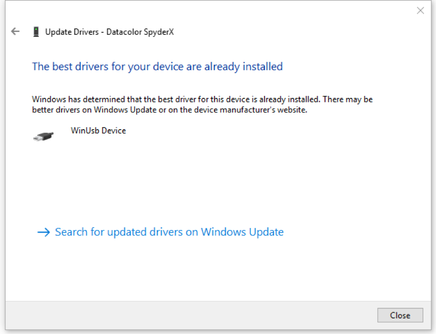
Figure 5. Installing the driver from a downloaded file in a folder.
2.4. Now, you will see a window showing "Installing drivers…" as the driver is being installed (Figure 6).
Note: On 64-bit Windows 8 or 10, you might not be able to install the driver because of the “driver signature enforcement” feature, as detailed in this link: https://www.howtogeek.com/167723/how-to-disable-driver-signature-verification-on-64-bit-windows-8.1-so-that-you-can-install-unsigned-drivers/
To resolve this issue, you can run the program provided in the package called “enableTestModeWin10.cmd” (right-click, choose “Run as administrator”) and then restart the computer. Follow Steps 2.1 to 2.4 above. After completing the installation of the Spyder driver as detailed above, you can then re-enable the “driver signature enforcement” feature by running the program called “disableTestModeWin10.cmd” (right click, choose “Run as administrator”) and then restart the computer.
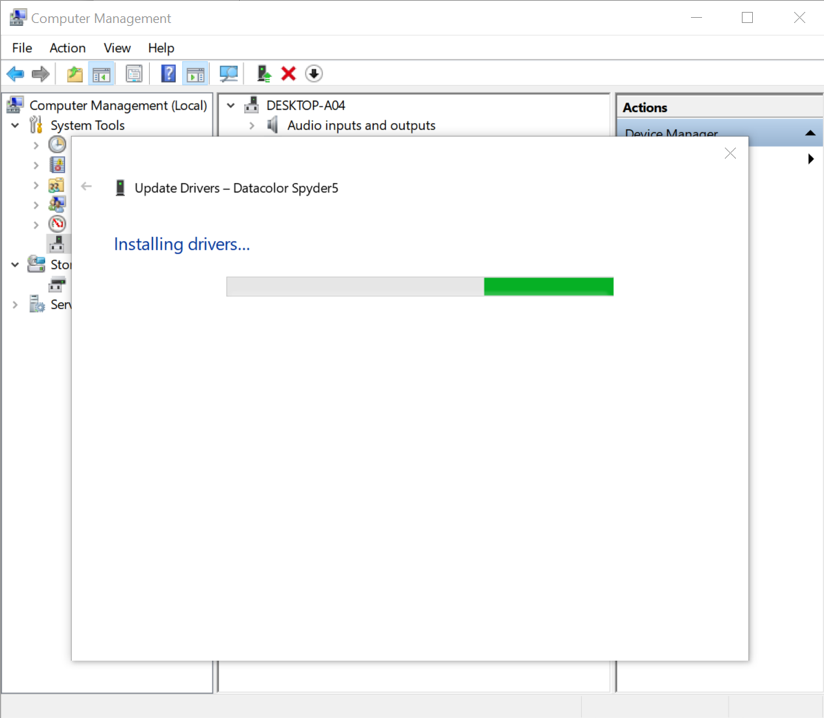
Figure 6. Driver installation in progress.
2.5. After the installation is complete, you will see a display showing "Windows has successfully updated your drivers" (Figure 7). If you go to the "Device Manager" setting, you will see that the driver has been installed, as shown in Figure 1.
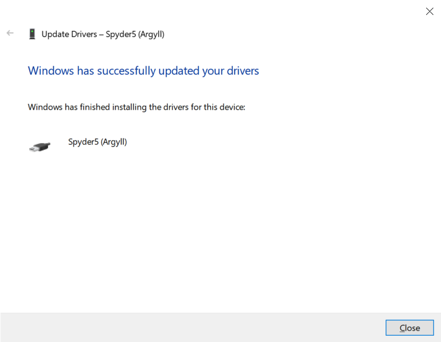
Figure 7. Driver installation completed.
We need to add the “PsyCalibrator” folder to MATLAB so that the included functions can be accessed within MATLAB. To do so, open the MATLAB software. Then, in the command window, add the “PsyCalibrator” folder to MATLAB by using the following command:
>> addpath(genpath(Path)); savepath;
Where “Path” should be replaced with the actual file path for PsyCalibrator in your computer, such as ‘D:/PsyCalibrator’ (as highlighted by Section 1 in Figure 8). Note that in this tutorial, the command text is colored blue; and variables that need to be changed are colored red; anything else, such as quotes that are not colored blue or red, should not be included in the command.
You only need to do this once—if you have already added the “PsyCalibrator” folder to MATLAB paths, you don’t need to do it again.
After the custom driver is installed, Spyder is ready to take measurements of luminance and color. To ensure accuracy, we first need to calibrate it, with two steps:
-
close the cover (if the cover is not on)
-
run the below command in MATLAB. Then hit any key to proceed. If successful, you will see the output “Calibration done!” within a second or two.
>> spyderCalibration_APL;
To measure the luminance/color of a stimulus on the monitor, simply open the cover and point the Spyder sensor closely to the target stimulus on the screen. Measurement is not limited to the stimuli on the screen—you can also use it to measure the luminance/color of things around you. For maximum accuracy and transparency, 1) make sure the sensor area is smaller than the stimulus, or else the measurement reflects not just the target stimulus but also the surrounding stimuli (if the target is too small, consider enlarging it); and 2) report the measurement distance (note that distance negatively affects luminance values if the object of interest is the sole or primary source of light).
Then run:
>> xyY = spyderRead_APL(refreshRate);
In which refreshRate is your display’s refresh rate number, such as 60 (HZ). The refresh rate describes how frequently your display refreshes the onscreen image. A 60 Hz screen refreshes images 60 times per second (i.e., every 16.67 ms). To find out the refresh rate, for Windows PCs, right-click on the desktop screen, click the “Display settings” icon, then click the “Advanced display settings” icon. For macOS, click on the Mac icon on the top left, click “About This Mac”; on the pop-out menu, open the “Displays” tap.
The returned xyY values are the CIE 1931 xyY color coordinates of the stimulus: xy for the coordinates in the color space that specify the color; Y (the third value) for the luminance value. The returned xyY matrix has five rows (for five measurements) and three columns (for xyY). To obtain the averaged measurement of xyY, run “xyY_mean = mean(xyY,1)”.
>> xyY_mean = mean(xyY,1);
The above steps are for luminance and color measurement. When a linear relation between RGB and luminance is convenient or necessary for your study, it’s time for display correction or calibration. To calibrate the display so that the RGB intensity and luminance relation is linear—either with respect to each individual color channel (that is, R, G, or B) or with respect to their average (that is, gray, with the same value in R, G, and B)—follow Steps 5 to 7, which illustrates the procedure for luminance calibration. The procedure can be adapted for individual RGB channel calibration—the only difference is the RGB channels (three channels vs. one channel).
Before calibration, make sure that no direct light shines on the monitor panel and that the monitor is turned on for at least 60 minutes to allow time for warm-up. When ready, follow the steps below to begin the calibration process.
5.1. Run the following command in MATLAB: "gammaMeasure_APL(deviceType)", where deviceType refers to the type of the Spyder device: 1 for Spyder5; and 2 for SpyderX. (For individual RGB channel calibration, use "gammaMeasure_APL(deviceType,[],[],[],[],[],[],2)".)
>> gammaMeasure_APL(deviceType,[],[],[],[],[],[],2);
5.2. In the command window, based on the prompts, you can optionally enter the relevant information of the display, including: brand, model, serial number, brightness, contrast, color temperature, computer brand, operating system, and graphics card (as highlighted by Section 2 in Figure 8). Providing this information is optional; you can press the Enter key to ignore these queries.
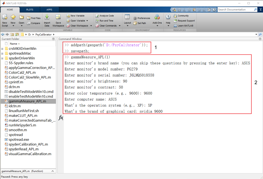
Figure 8. MATLAB command window.
5.3. After the above step, press the "Enter" key. Now, the program will start the calibration process by opening a new window (Figure 9). As indicated by the instruction on this window, before measuring the display, we need to calibrate the device itself first, by closing the lens cover (as in luminance measurement in Step 4). This calibration process lasts only a few seconds. Then press any key to start the measurement.
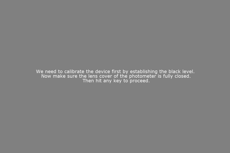
Figure 9. Photometer calibration window.
5.4. After the equipment itself has been calibrated, the program is now ready to take measurements of a series of images automatically (Figure 10). At this time, turn off the lights in the room, and point the sensor of the photometer directly to the screen at the intersection of the two diagonal lines in Figure 10. The lens cover of the Spyder device can hang on the back of the display as a counterweight to keep balance. After completing this setup, press any key to continue.
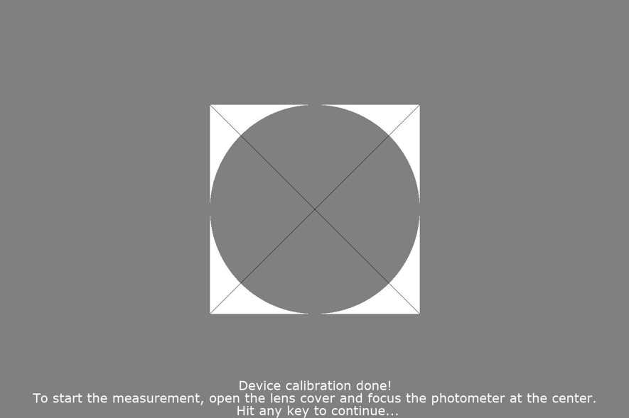
Figure 10. Begin the measurement process.
5.5. Because ambient light can affect the measurement, it is recommended that the light level be constant. So if the room needs to be very dark and you need to turn on the light to leave the room, do so within 10 seconds (Figure 11), after which the photometer will take measurements by itself (the 10 seconds delay is determined by the input parameter LeaveTime in gammaMeasure_APL).
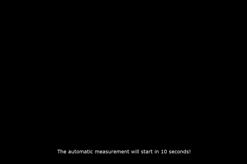
Figure 11. Automatic measurement starts within 10 seconds.
5.6. During the measurement, a series of uniform square images will appear on the screen automatically while the photometer reads its luminance level (Figure 12).

Figure 12. Uniform square images on the screen.
5.7. After the calibration is completed, a file that contains the measurement results will be generated in MATLAB within the current working path, named Gamma.mat (as highlighted in Figure 13).
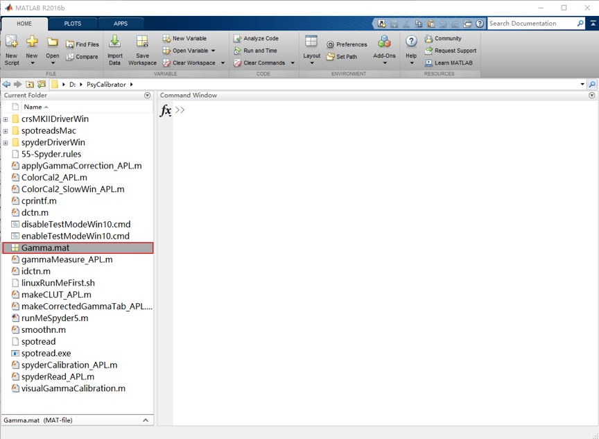
Figure 13. The calibration results are saved to the file name Gamma.mat.
To linearize the display, PsyCalibrator incorporates the Mcalibrator2 toolkit an (Ban & Yamamoto, 2013) to fit the data. Specifically, Mcalibrator2 implements several data fitting methods that do not assume the specific relation between video input and luminance output of the display (such as the gain-offset-gamma model or the gain-offset-gamma-offset model often assumed in CRT displays). These data-driven, model-free fitting methods can provide a better fit for various types of displays, from CRT to LCD and projectors, resulting in better linear correction. In our case, we mainly use the cubic spline interpolation method as it generally provides a superior fit.
6.1. To fit the measurement data, enter and execute the following command in MATLAB:
>> Gamma = makeCorrectedGammaTab_APL('Gamma.mat');
The fitting result is saved to a new file within the same directory, named Gamma_fitted.mat, along with a figure visualizing the result (Figure 15). The generated file contains a structural variable named Gamma, in which Gamma.gammaTable (highlighted by Section 2 in Figure 14) is the color lookup table (CLUT, which translates the colors in an image to the colors in the hardware). As detailed in Step 7, CLUT is then used for linearization, specifying the midpoint RGB intensity level that corresponds to the midpoint luminance level, and so on.
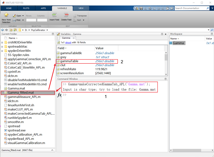
Figure 14. Data fitting and results.
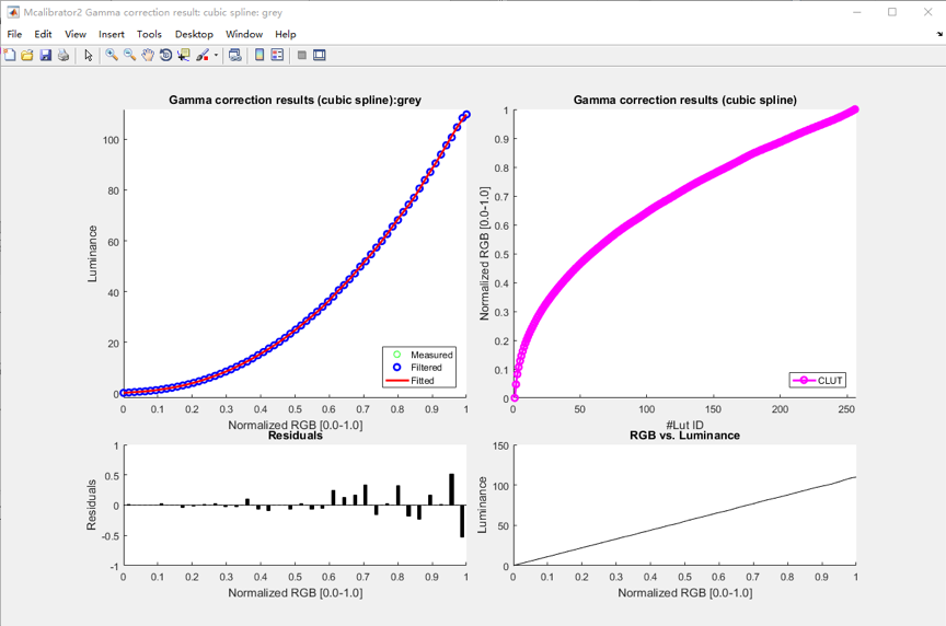
Figure 15. Video input and luminance relation.
6.2. To verify the linearity of the display with the fitted CLUT, we need to measure the relation between RGB intensity and luminance with a photometer. As highlighted in Figure 16, to do so, execute the function gammaMeasure_APL as used before for luminance measurement (replace deviceType with the correct device type):
>> gammaMeasure_APL(deviceType,[],[],[],Gamma.gammaTable);
where deviceType refers to the type of test device: 1 for Spyder5 and 2 for SpyderX. The procedure is the same as in Steps 5.2 to 5.7 above. Finally, the results are saved to the file “Gamma_verification.mat” (Figure 17). Linearity is visualized with a figure showing the relation between RGB and luminance (from the variable xyY in Gamma_verification.mat; Figure 18). For color channel calibration, use:
>> gammaMeasure_APL(deviceType,[],[],[], Gamma.gammaTable,[],[],2);
The rest is similar.
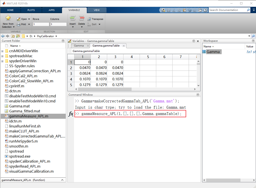
Figure 16. Verify the linearity of the display after applying the CLUT.
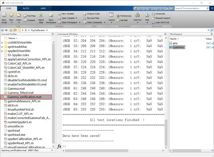
Figure 17. Verification results are saved to the file Gama_verification.mat.
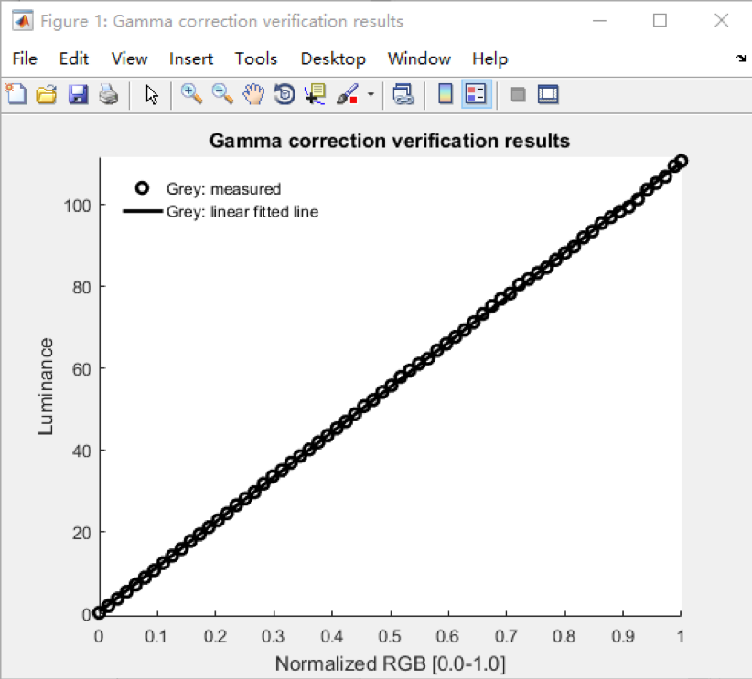
Figure 18. Visualization of the linearity of the display after applying the CLUT.
With the CLUT from the last step, we can use it for gamma correction (that is, to linearize the display). Afterward, we can also restore the display to its uncorrected state. This is implemented using a function called applyGammaCorrection_APL. This function has three input parameters. The first parameter (0 or 1) concerns the action of the function: 0 means no gamma correction (i.e., the default); 1 means applying the gamma correction. The second parameter is the CLUT to be applied (that is, Gamma.gammaTable from Step 6.1 for correction). The third parameter is the specific monitor that we would like to apply the correction to (see http://psychtoolbox.org/docs/Screen-Screens).
Therefore, for example, to perform gamma correction for the monitor numbered 0 based on Gamma.gammaTable, execute the following command in MATLAB:
>> applyGammaCorrection_APL(1, Gamma.gammaTable,0);
To remove the correction (that is, to restore the display to its default status), execute:
>> applyGammaCorrection_APL(0, [], 0);
Ban, H., & Yamamoto, H. (2013). A non-device-specific approach to display characterization based on linear, non-linear, and hybrid search algorithms. Journal of vision, 13(6):20, 1–26.