EE8204---Real-Time-Multi-Task-Learning

Real-Time Joint Semantic Segmentation and Depth Estimation Using Asymmetric Annotations Implementation

Summary

This repository provides a python implementation using PyTorch for the following research paper: Title: Real-Time Joint Semantic Segmentation and Depth Estimation Using Asymmetric Annotations Link: https://arxiv.org/abs/1809.04766

This page will serve as a guide to explain the paper, but also to walk anyone interested in the paper through the steps needed to implement the network in python. Currently the implementation us in PyTorch but in the future I would like to convert the implementation to TensorFlow.

Intro

The focus of this paper is to accomplish semantic segmentation and depth estimation using asymmetrical data sets. An asymmetrical data set is simply a data set that contains labels for one of the tasks but not all of them. In the case of this paper the data sets used are the NYUDv2 indoor and KITTI outdoor images. The data set images may have labelled data referencing the semantic map or the depth information.

In order to accomplish the goal of performing both semantic segmentation and depth estimation the author of the paper V. Nekrasov et al. utilizes the following two techniques:

1. Multi-task Learning - Used to create a network that can accomplish both Semantic Segmentation and Depth Estimation
2. Knowldge Distillation - Used to estimate missing label information in data sets based on expert pre-trained teacher network

Data Sets Used to Train the weights A previous network was used with the NYUDv2 and KITTI outdoor data sets to pre-train the weights. These weights were then used in this implementation to show how the network can quickly perform semantic segmentation and depth estimation.

Dependencies

• --find-links https://download.pytorch.org/whl/torch_stable.html
• torch===1.6.0
• torchvision==0.7.0
• numpy
• opencv-python
• jupyter
• matplotlib
• Pillow

Network Architecture

The network architecture found in this paper can be broken down into four major parts:

1. Encoder Network
2. Light-Weight Refine Network
3. Chained Residual Pooling blocks
4. Task specific Convolution
   • Segmentation
   • Depth Estimation

A visual summary of the network architecture is provided below directly from the paper.

The Encoder network is built from the ResNet architecture and supports ResNet [50, 101, 152]. The ResNet architecutre for the 34 layer network is shown below.

The ResNet architecture employees residual learning which in short is a skip connection that allows the input to a group of layers to skip and be added back to the output of that layer. This can be visualized as mathematically as F(x) + x where x is the input image and F(x) if the input image after convolution-batch normalization-activation have been perform (possibly also pooling for up/down sampling).

The encoder network (ResNet) can be broken down into smaller chunks as seen in the ResNet 34 architecutre. The basics for a 34 layer ResNet are:

1.Input Image - 224 x 224 x 3 image (RGB)

2. Convolution Layer 1 (grouping layer 1)

   • Input: Input image
     • Input image = x
   • Conv: 7x7 kernel, 64 feature maps, stride 2, padding = 3
     • size = 112 x 112 x 64 (row x column x feature maps)
   • Batch normalization
   • Max Pooling, stride 2
     • size = 56 x 56 x 64 (row x column x feature maps)
   • Output: Grouping1_Conv_1
     • size = 56 x 56 x 64 (row x column x feature maps)
     • let Grouping1_Conv1 = x_G1

3. Convolution Layer 2 (grouping layer 2)

   • Input: Grouping1_Conv_1, skip connection to after 2 convolutional layers
     • Input: x_1 = x_G1
   • Conv: 3x3 kernel, 64 feature maps, stride 1, padding = 1
     • size = 56 x 56 x 64 (row x column x feature maps)
   • Conv: 3x3 kernel, 64 feature maps, stride 1, padding = 1
     • size = 56 x 56 x 64 (row x column x feature maps)
   • Output: Output_after_2_convolutions + Grouping1_Conv_1
     • Let the output after two convolutions be F1(x) = x_G2_Conv1
     • Output of skip connection is H1(x) = F1(x) + x_1
     • H1(x) = x_G2_Conv1 + x_G1
     • Let H1(x) = x_G2_SL1
   • Input: Output of previous skip connection H1(x) = x_G2_SL1, skip connection to after 2 convolutional layers
     • Input: x_2 = x_G2_SL1
   • Conv: 3x3 kernel, 64 feature maps, stride 1
     • size = 56 x 56 x 64 (row x column x feature maps)
   • Conv: 3x3 kernel, 64 feature maps, stride 1
     • size = 56 x 56 x 64 (row x column x feature maps)
   • Output: Output_after_2_convolutions + x_G2_SL1
     • Let the output after two convolutions be F2(x) = x_G2_Conv2
     • Output of skip connection is H2(x) = F2(x) + x_2
     • H2(x) = x_G2_Conv2 + x_G2_SL1
     • Let H2(x) = x_G2_SL2
   • Input: Output of previous skip connection H2(x) = x_G2_SL2, skip connection to after 2 convolutional layers
     • Input: x_3 = x_G2_SL2
   • Conv: 3x3 kernel, 64 feature maps, stride 1
     • size = 56 x 56 x 64 (row x column x feature maps)
   • Conv: 3x3 kernel, 64 feature maps, stride 1
     • size = 56 x 56 x 64 (row x column x feature maps)
   • Output: Output_after_2_convolutions + x_G2_SL2
     • Let the output after two convolutions be F3(x) = x_G2_Conv3
     • Output of skip connection is H3(x) = F3(x) + x_3
     • H3(x) = x_G2_Conv3 + x_G2_SL2
     • Let H3(x) = x_G2_SL3

4. Convolution Layer 3 (Grouping Layer 3)

   • Input: Output of previous skip connection H3(x) = x_G2_SL3, skip connection to after 2 convolutional layers
     • Input: x_4 = x_G2_SL3
   • Conv: 3x3 kernel, 128 feature maps, stride 2
     • size = 28 x 28 x 128 (row x column x feature maps)
   • Conv: 3x3 kernel, 128 feature maps, stride 1
     • size = 28 x 28 x 128 (row x column x feature maps)
   • Output: Output_after_2_convolutions + x_G2_SL3
     • Let the output after two convolutions be F4(x) = x_G3_Conv1
     • Output of skip connection is H4(x) = F4(x) + x_4
     • H3(x) = x_G3_Conv1 + x_G2_SL3
     • Let H4(x) = x_G3_SL1
   • Input: Output of previous skip connection H4(x) = x_G3_SL1, skip connection to after 2 convolutional layers
     • Input: x_5 = x_G3_SL1
   • Conv: 3x3 kernel, 128 feature maps, stride 1
     • size = 28 x 28 x 128 (row x column x feature maps)
   • Conv: 3x3 kernel, 128 feature maps, stride 1
     • size = 28 x 28 x 128 (row x column x feature maps)
   • Output: Output_after_2_convolutions + x_G3_SL1
     • Let the output after two convolutions be F5(x) = x_G3_Conv2
     • Output of skip connection is H5(x) = F5(x) + x_5
     • H5(x) = x_G3_Conv2 + x_G3_SL1
     • Let H5(x) = x_G3_SL2
   • Input: Output of previous skip connection H5(x) = x_G3_SL2, skip connection to after 2 convolutional layers
     • Input: x_6 = x_G3_SL2
   • Conv: 3x3 kernel, 128 feature maps, stride 1
     • size = 28 x 28 x 128 (row x column x feature maps)
   • Conv: 3x3 kernel, 128 feature maps, stride 1
     • size = 28 x 28 x 128 (row x column x feature maps)
   • Output: Output_after_2_convolutions + x_G3_SL2
     • Let the output after two convolutions be F6(x) = x_G3_Conv3
     • Output of skip connection is H6(x) = F6(x) + x_6
     • H6(x) = x_G3_Conv3 + x_G3_SL2
     • Let H6(x) = x_G3_SL3
   • Input: Output of previous skip connection H6(x) = x_G3_SL3, skip connection to after 2 convolutional layers
     • Input: x_7 = x_G3_SL3
   • Conv: 3x3 kernel, 128 feature maps, stride 1
     • size = 28 x 28 x 128 (row x column x feature maps)
   • Conv: 3x3 kernel, 128 feature maps, stride 1
     • size = 28 x 28 x 128 (row x column x feature maps)
   • Output: Output_after_2_convolutions + x_G3_SL3
     • Let the output after two convolutions be F7(x) = x_G3_Conv4
     • Output of skip connection is H6(x) = F7(x) + x_7
     • H7(x) = x_G3_Conv4 + x_G3_SL3
     • Let H7(x) = x_G3_SL4

5. Convolution Layer 4 (Grouping Layer 4)

   • Input: Output of previous skip connection H7(x) = x_G3_SL4, skip connection to after 2 convolutional layers
     • Input: x_8 = x_G3_SL4
   • Conv: 3x3 kernel, 256 feature maps, stride 2
     • size = 14 x 14 x 256 (row x column x feature maps)
   • Conv: 3x3 kernel, 256 feature maps, stride 1
     • size = 14 x 14 x 256 (row x column x feature maps)
   • Output: Output_after_2_convolutions + x_G3_SL4
     • Let the output after two convolutions be F8(x) = x_G4_Conv1
     • Output of skip connection is H8(x) = F8(x) + x_8
     • H8(x) = x_G4_Conv1 + x_G3_SL4
     • Let H8(x) = x_G4_SL1
   • Input: Output of previous skip connection H8(x) = x_G4_SL1, skip connection to after 2 convolutional layers
     • Input: x_9 = x_G4_SL1
   • Conv: 3x3 kernel, 256 feature maps, stride 1
     • size = 14 x 14 x 256 (row x column x feature maps)
   • Conv: 3x3 kernel, 256 feature maps, stride 1
     • size = 14 x 14 x 256 (row x column x feature maps)
   • Output: Output_after_2_convolutions + x_G4_SL1
     • Let the output after two convolutions be F9(x) = x_G4_Conv2
     • Output of skip connection is H9(x) = F9(x) + x_9
     • H9(x) = x_G4_Conv2 + x_G4_SL1
     • Let H9(x) = x_G4_SL2
   • Input: Output of previous skip connection H9(x) = x_G4_SL2, skip connection to after 2 convolutional layers
     • Input: x_10 = x_G4_SL2
   • Conv: 3x3 kernel, 256 feature maps, stride 1
     • size = 14 x 14 x 256 (row x column x feature maps)
   • Conv: 3x3 kernel, 256 feature maps, stride 1
     • size = 14 x 14 x 256 (row x column x feature maps)
   • Output: Output_after_2_convolutions + x_G4_SL2
     • Let the output after two convolutions be F10(x) = x_G4_Conv3
     • Output of skip connection is H10(x) = F10(x) + x_10
     • H10(x) = x_G4_Conv3 + x_G4_SL2
     • Let H10(x) = x_G4_SL3
   • Input: Output of previous skip connection H10(x) = x_G4_SL3, skip connection to after 2 convolutional layers
     • Input: x_11 = x_G4_SL3
   • Conv: 3x3 kernel, 256 feature maps, stride 1
     • size = 14 x 14 x 256 (row x column x feature maps)
   • Conv: 3x3 kernel, 256 feature maps, stride 1
     • size = 14 x 14 x 256 (row x column x feature maps)
   • Output: Output_after_2_convolutions + x_G4_SL3
     • Let the output after two convolutions be F11(x) = x_G4_Conv4
     • Output of skip connection is H11(x) = F11(x) + x_11
     • H11(x) = x_G4_Conv4 + x_G4_SL3
     • Let H11(x) = x_G4_SL4
   • Input: Output of previous skip connection H11(x) = x_G4_SL4, skip connection to after 2 convolutional layers
     • Input: x_12 = x_G4_SL4
   • Conv: 3x3 kernel, 256 feature maps, stride 1
     • size = 14 x 14 x 256 (row x column x feature maps)
   • Conv: 3x3 kernel, 256 feature maps, stride 1
     • size = 14 x 14 x 256 (row x column x feature maps)
   • Output: Output_after_2_convolutions + x_G4_SL4
     • Let the output after two convolutions be F12(x) = x_G4_Conv5
     • Output of skip connection is H12(x) = F12(x) + x_12
     • H12(x) = x_G4_Conv5 + x_G4_SL4
     • Let H12(x) = x_G4_SL5
   • Input: Output of previous skip connection H12(x) = x_G4_SL5, skip connection to after 2 convolutional layers
     • Input: x_13 = x_G4_SL5
   • Conv: 3x3 kernel, 256 feature maps, stride 1
     • size = 14 x 14 x 256 (row x column x feature maps)
   • Conv: 3x3 kernel, 256 feature maps, stride 1
     • size = 14 x 14 x 256 (row x column x feature maps)
   • Output: Output_after_2_convolutions + x_G4_SL5
     • Let the output after two convolutions be F13(x) = x_G4_Conv6
     • Output of skip connection is H13(x) = F13(x) + x_13
     • H13(x) = x_G4_Conv6 + x_G4_SL5
     • Let H13(x) = x_G4_SL6

6. Convolution Layer 5 (Grouping Layer 5)

   • Input: Output of previous skip connection H13(x) = x_G4_SL6, skip connection to after 2 convolutional layers
     • Input: x_14 = x_G4_SL6
   • Conv: 3x3 kernel, 512 feature maps, stride 2
     • size = 7 x 7 x 512 (row x column x feature maps)
   • Conv: 3x3 kernel, 512 feature maps, stride 1
     • size = 7 x 7 x 512 (row x column x feature maps)
   • Output: Output_after_2_convolutions + x_G4_SL6
     • Let the output after two convolutions be F14(x) = x_G5_Conv1
     • Output of skip connection is H14(x) = F14(x) + x_14
     • H14(x) = x_G5_Conv1 + x_G4_SL6
     • Let H14(x) = x_G5_SL1
   • Input: Output of previous skip connection H14(x) = x_G5_SL1, skip connection to after 2 convolutional layers
     • Input: x_15 = x_G5_SL1
   • Conv: 3x3 kernel, 512 feature maps, stride 1
     • size = 7 x 7 x 512 (row x column x feature maps)
   • Conv: 3x3 kernel, 512 feature maps, stride 1
     • size = 7 x 7 x 512 (row x column x feature maps)
   • Output: Output_after_2_convolutions + x_G5_SL1
     • Let the output after two convolutions be F15(x) = x_G5_Conv2
     • Output of skip connection is H15(x) = F15(x) + x_15
     • H15(x) = x_G5_Conv2 + x_G5_SL1
     • Let H15(x) = x_G5_SL2
   • Input: Output of previous skip connection H15(x) = x_G5_SL2, skip connection to after 2 convolutional layers
     • Input: x_16 = x_G5_SL2
   • Conv: 3x3 kernel, 512 feature maps, stride 1
     • size = 7 x 7 x 512 (row x column x feature maps)
   • Conv: 3x3 kernel, 512 feature maps, stride 1
     • size = 7 x 7 x 512 (row x column x feature maps)
   • Output: Output_after_2_convolutions + x_G5_SL2
     • Let the output after two convolutions be F16(x) = x_G5_Conv3
     • Output of skip connection is H16(x) = F16(x) + x_16
     • H16(x) = x_G5_Conv3 + x_G5_SL3
     • Let H16(x) = x_G5_SL3

7. Average Pooling (Global Average Pooling)

   • Global Average Pooling is applied to the output of the last convolutional grouping in the ResNet 34. This global average pooling takes the 7 x 7 x 512 tensor of feature maps and averages the 7 x 7 feature map into a 1 x 1 feature map of depth 512. The output of this layer is a feature map of 1 x 1 x 512.

8. Full Connected Layer

   • The Global Average Pooling is the connected to each output neuron. Each feature map in the 1 x 1 x 512 is connected to the output neurons making this a fully connected layer.

The ResNet 34 architecutre shown above can be extended to 50/101/152 layers. This example is just to illustrate the encoder architecutre used in the paper. The different ResNet architecutres can all be used to determine which architecture gives the best results. For each ResNet architecture the decoder architecture which uses the Light Weight RefineNet will need to be updated.

The encoder passes the output directly to the Light Weight RefineNet at the output of the encorder and through chained residual pooling blocks. The Light Weight RefineNet implementation is used as a decoder with an architecture as described in the following paper https://arxiv.org/pdf/1810.03272.pdf where modification are made to the original RefineNet to make it more desirable for real time semantic segmentation. A basic idea of the architecture is shown in the picture below:

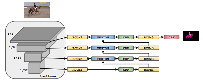
The main changes found in this paper to the architecutre of the Light Weight Refine Network is the changing of the Residual Convolution Units (RCU) that connect the output of each encoder feature map to the decoder are now Chained Residual Pooling (CRP) blocks. This means that at the input of each decoder layered grouping the corresponding feature map from the encoder will pass throught the CRP blocks before beginning the process of following the Light Weight Refine Network architecutre of passing through a light weight fusion block, leight weight CRP block, and a leight weight RCU block before all being added together to create an output image the same size as the input image.

Finally, the paper makes use of two task branches at the output of the Light Weight Refine Network. Each branch has the same architecture with a 1x1 depth convolution and a 3x3 convolution. Using Multitask learning each branch is able to perform a signle task such as semantic segmentation and depth estimation.

Paper Implementation

How to run the code In order to get this code to run I recommend copying the entire repository to your local drive. Create a folder and then use the python venv function to create a local copy of the python interpreter.

The dependencies for this project will be listed below. This specific implementation was done in windows 7 ultimate 64 bit. Using a pretrained network for real time semantic segmentation and depth estimation. The pre trained network can be found in the weights folder. It is possible to pre-train a netowkr with specific weights using a different architecture but in this implementation I decicded to follow the original authors methodoolgy to try and get results as close as possibly to the original paper.

Exmaple of projecy directory creation in command line:

mkdir my_Project
-m venv my_Project\venv

Extract this repositor to within the folder you created but do not place the venv folder. Once the requirements.txt folder is in your selected folder run the following command in command prompt to download the required libraries/frameworks:

my_Project\venv\Scripts\activate.bat
pip install -r requirements.txt

Once all the dependencies are installed you will be able to add aditional images to the examples folder and then upadate the folder path within the evaluation python file by changing the img_Path variable to have the associated path to your new image.

This implementation makes use of check point files and pretrained weights for the network. The pretrained weights are determined by using the Light Weight Refine Net with a ResNet encoder to determine the optimal weights for semantic segmentation. Then the new network built specifically for this paper makes use of those weights and multi task learning to accurately guess the missing label data for either semantic mapping or depth estimation.

Conclusions

This paper provides a deep dive for the reader if they want to become familiar with encoder decoder networks, ResNet, RefineNet and Leight Weight Refine Net. Using pretrained wieghts significantly speeds up the time to process an input image into is respective semantic and depth mapping. A full pipeline implementation from ResNet to Light Weight Refine net is the next goal of work to test the real-time capabilities of this method from start to finish.

The ease with which the network performs multi-task learning using the pre-train weights is a great indicator of possible future work. Aside from the full pipe line implementation it would be interesting to try and change the network architecture to use different encoder and decoders to see if this method can stil be improved.