TravelModel1.5
Home > TravelModel > Development > TravelModel1.5
Travel Model 1.5 is a major update to MTC's Activity-Based Travel Model One. It was developed for the Horizon initiative, so it added representation for:
- ride-hailing (or Transportation Network Company - TNC) and taxi modes
- autonomous vehicles
TM1.5 tour and trip-based mode choice models were modified to explicitly represent the choice of Taxi and Transportation Networking Company (TNC) modes (also known as ride-hailing). A new Taxi\TNC nest was added with sub-alternatives for traditional taxi versus new TNC modes including single-party TNC (e.g. uberX) versus shared TNC (e.g. uberPOOL). These capabilities provide the analyst with the ability to represent different assumptions about taxi and TNC actual and/or perceived times and costs, and observe changes in mode shares related to these assumptions. The analyst may additionally need to specify alternative-specific constants related to transformative mobility changes related to the introduction of AVs. This is particularly true if a future is envisioned in which auto ownership changes substantially due to the proliferation of AV technology and significantly greater availability of TNCs. For example, significantly increasing the number of 0-auto households would likely result in much higher shares of transit trips in the current model, since 0-auto households currently generate a significant proportion of transit trips. However, if the assumption is that auto ownership will decrease due to increased availability of private and/or TNC fleets of AVs, the mode choice model would also need to be calibrated to reflect this assumption. In such cases, the user may need to introduce alternative specific constants to reflect assumptions about changes in mode.
The table below shows the utility components associated with Taxi and TNC modes.
| Utility Component | Variable - Taxi | Variable - TNC | Coefficient |
|---|---|---|---|
| In-vehicle time | Shared-2 Toll/HOV time | Shared-2 Toll/HOV time | Generic in-vehicle coefficient |
| Wait time | Simulated from distribution (described below) | Simulated from distribution (described below) | 1.5 * IVT coefficient |
| Tolls | Shared-2 Toll/HOV toll (if any) | Shared-2 Toll/HOV toll (if any) | Generic cost coefficient |
| Bridge toll | Shared-2 Toll/HOV bridge tolls (if any) | Shared-2 Toll/HOV bridge tolls (if any) | Generic cost coefficient |
| Fare | Initial cost + cost per mile * distance + cost per minute * time | Max(minCost, Initial cost + cost per mile * distance + cost per minute * time) | Generic cost coefficient |
| Alternative-specific constant | Base year = calibrated Future-year = User-defined |
Base year = unavailable Future-year = User-defined |
N.A. |
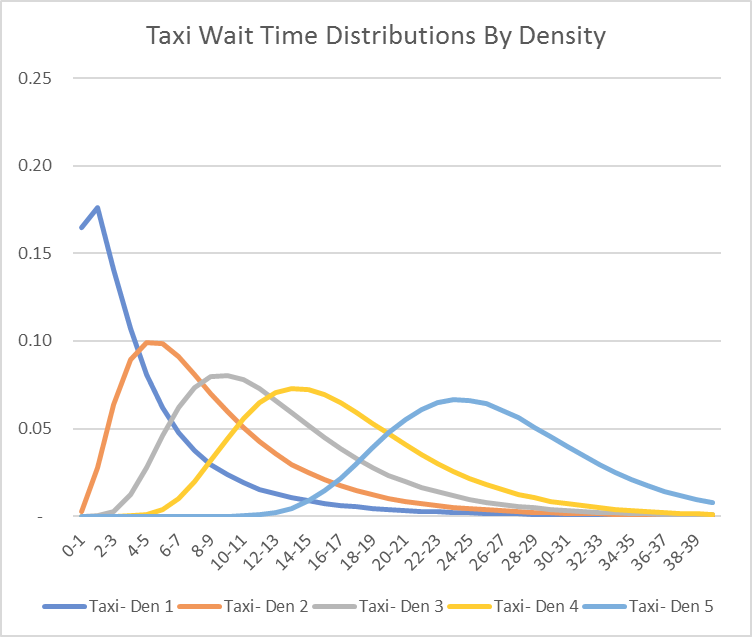
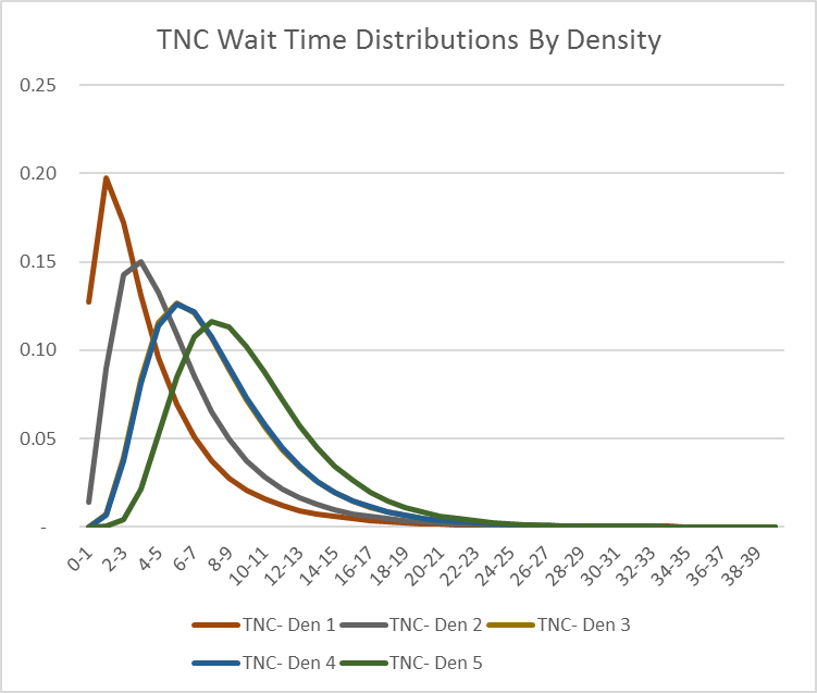
Taxi and TNC mode wait times are simulated from distributions that were estimated based on a survey of actual taxi and TNC wait times conducted in the Portland region in 2015 (see https://www.portlandmercury.com/images/blogimages/2015/07/10/1436550157-uber_taxi_report.pdf). The survey data was limited to call-initiated pickups (no pre-planned pickups were included). Lognormal distributions were estimated from this observed data for each mode according to the land-use density of the tour or trip origin. Density is defined as (population + employment)/area (sq. mi.). There are five categories of density from high to low with breakpoints at 15000, 5000, 2000, and 500.
The wait time distributions for taxi trips and TNCs are shown in the figures below, with average wait times shown in the table. As shown in the figures and tables, the ranges of wait time and standard deviation for taxi are much higher for taxis than for TNCs. Even so, the average wait time for a TNC for trips starting in the lowest density bin was over 10 minutes in 2015. This wait time may decrease in the future as demand for TNCs increase. The wait times for Shared TNC were asserted since the Portland data does not split out Shared from Single ride TNCs.
| Density Range | Average Wait Time (min) | |||
|---|---|---|---|---|
| High | Low | Taxi | TNC-Single | TNC-Shared |
| 100000000 | 15000 | 5.5 | 4.7 | 7.0 |
| 15000 | 5000 | 9.5 | 6.3 | 8.0 |
| 5000 | 2000 | 13.3 | 8.4 | 11.0 |
| 2000 | 500 | 17.3 | 8.5 | 15.0 |
| 500 | 0 | 26.5 | 10.3 | 15.0 |
Since the average and standard deviation of each lognormal distribution could change in the future, they are user-defined properties in the params.properties file and can be varied with respect to specific scenarios.
#Note: the following comma-separated value properties cannot have spaces between them, or else the RuntimeConfiguration.py code won't work
TNC.single.waitTime.mean = 10.3,8.5,8.4,6.3,4.7
TNC.single.waitTime.sd = 4.1,4.1,4.1,4.1,4.1
TNC.shared.waitTime.mean = 15.0,15.0,11.0,8.0,7.0
TNC.shared.waitTime.sd = 4.1,4.1,4.1,4.1,4.1
Taxi.waitTime.mean = 26.5,17.3,13.3,9.5,5.5
Taxi.waitTime.sd = 6.4,6.4,6.4,6.4,6.4
TNC and taxi cost variables are also set in the params.properties file, with base-year values set based on publicly available data (link= http://uberestimate.com/). The base-year costs are shown in the table below. In future year AV scenarios, the TNC cost can be adjusted down to reflect the decrease in labor costs associated with driverless cars.
| Cost Component | Taxi | TNC - Single | TNC-Shared* |
|---|---|---|---|
| Base Fare | $2.20 | $2.20 | $2.20 |
| Cost per mile | $2.30 | $1.33 | $0.44 |
| Cost per minute | $0.10 | $0.24 | $0.08 |
| Minimum cost per trip | 0 | $7.20 | $3.00 |
taxi.baseFare = 2.20
taxi.costPerMile = 2.30
taxi.costPerMinute = 0.10
TNC.single.baseFare = 2.20
TNC.single.costPerMile = 1.33
TNC.single.costPerMinute = 0.24
TNC.single.costMinimum = 7.20
# use lower costs for TNC shared
TNC.shared.baseFare = 2.20
TNC.shared.costPerMile = 0.44
TNC.shared.costPerMinute = 0.08
TNC.shared.costMinimum = 3.00
Additionally, there is an in-vehicle time multiplier for Shared TNCs to reflect out-of-direction travel to pick-up or drop-off additional customers.
# Based on data collected in Chicago between Nov 2017 to Mar 2018 (Schwieterman and Livingston, 2018)
Mobility.TNC.shared.IVTFactor = 1.5The vehicle occupancy factors for taxis, single TNCs, and shared TNCs are shown below. These factors add up to 1.0 across all occupancies (da = drive alone, s2 = shared-ride 2 occupant, s3 = shared-ride 3+ occupant). They are multiplied by the total trips in each mode to determine trips by mode and occupancy.
See source
# vehicle occupancy for TNC and Taxi
Taxi.da.share = 0.00
Taxi.s2.share = 0.53
Taxi.s3.share = 0.47

TNC.single.da.share = 0.0
TNC.single.s2.share = 0.53
TNC.single.s3.share = 0.47

TNC.shared.da.share = 0.00
TNC.shared.s2.share = 0.18
TNC.shared.s3.share = 0.82Taxi, Single TNC, and Shared TNC are new modes in tour and trip output files (modes 19, 20, and 21 respectively). Taxi trips are currently allocated to drive-alone, shared-2, and shared 3+ modes according to a set of factors specified in the params.properties file. Single and Shared TNC trips are allocated to a combined set of additional AV and TNC trip tables according to a similar set of occupancy factors. These additional trip tables are then assigned separately using their respective value-toll eligible path, and a set of PCE factors that can be modified to reflect different passenger car equivalents for AVs versus HVs by facility type.
Several new components were introduced into the CT-RAMP model in TM1.5 to explicitly model the ownership and availability of autonomous vehicles (AVs). Because the level of private Autonomous Vehicle ownership and effects on total auto ownership, mode choice, destination choice, and congestion impacts are largely unknown, the approach that has been adopted is to provide the user with significant flexibility in how to represent the impacts of AVs. This type of modeling, called ‘scenario modeling’, requires the user to make some assumptions about how the future might look in terms of AV ownership, differences in perceived and/or actual time and cost of AVs versus human-controlled vehicles (HVs), and impacts on congestion. Then the user must translate those assumptions into model parameters so that the model outcomes reflect those assumptions. Typically, the model is run many times with systematically varied assumptions to test the effects of the ranges of assumptions on outcomes. This is typically referred to as _risk analysis_.
The following changes were made to enable this type of scenario modeling in TM 1.5. First, the auto ownership model was extended to consider autonomous (AV) versus human-controlled (HV) vehicles. Second, a simulation model was added that determines for each AV-owning household whether an AV is available for each tour. Third, the tour and trip mode choice models were modified to introduce user-defined coefficients and alternative-specific constants to represent AV-scenario assumptions. Fourth, the software was modified to explicitly track whether an AV was chosen for each tour and trip and to provide the capability to assign AVs as a separate vehicle class.
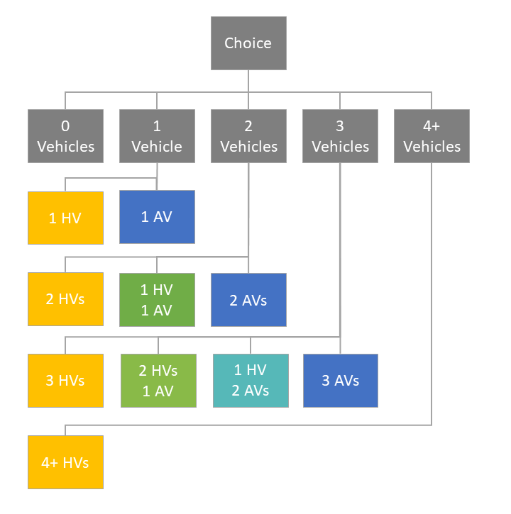
As shown in the figure below, the auto ownership model was extended to consider the number of AVs versus HVs for each auto-owning choice. This provides the capability to test different private AV ownership levels on downstream choices such as mode choice, and to track AV trios in separate trip tables. The AV versus HV nesting coefficient was asserted to be 0.5. It is assumed that a household owning 4 vehicles would likely not own any autonomous vehicles and future scenarios that assume high levels of AV ownership would significantly reduce or even eliminate the share of 4+ vehicle owning households.
The table below shows the coefficients added to the auto ownership model to capture likely socio-economic and mobility attributes related to AV ownership. The exponentiated values are also shown in order to illustrate the effect of the coefficient on the probability of AV ownership. These coefficients were adopted from recent AV scenario testing conducted by RSG using the Jacksonville DaySim model. They assume that younger and more wealthy households are more likely to own AVs, all else being equal; however, after discussion with partner agencies, MTC dropped age-related AV terms from the auto ownership model. They also assume that households with longer work commutes would be more likely to own an AV. Although they are informed by current literature, there is no way to statistically estimate these variables since there are no AV-owning households currently.
| Variable | Coefficient | exp(Coefficient) |
|---|---|---|
| Household Income under $50k | -1.0000 | 0.37 |
| Household Income 100k+ | 1.0000 | 2.72 |
| Hours of travel by auto for work, summed across all workers in household | 0.2500 | 1.28 |
In addition to these variables, a set of alternative-specific constants were applied and calibrated to reflect different levels of AV ownership according to scenario-specific targets. A spreadsheet was developed to calculate the target for each auto ownership choice based on a user-specified average vehicle ownership and a user-specified AV percentage of privately-owned vehicles. Calibration constants were developed for the three Horizon future scenarios (Clean and Green, Back to the Future, and Rising Tides Falling Fortunes) based upon the AV shares defined for those futures. The application of the constants are controlled by setting a parameter, Mobility.AV.Share, in the params.properties file. The value of this parameter is used to apply a different set of alternative specific constants to reflect shares of vehicles by auto ownership category and AV versus HV split. Future-specific versions of the params.properties file are posted on GitHub
Households that own at least one of each type of vehicle (HV and AV) have a choice of which vehicle to use for each tour, which is taken into account not only when auto is the chosen mode but also when evaluating other modal options (walk, bike, transit, etc.). TM1.5 was enhanced to make this decision explicit, without introducing a full vehicle allocation model that would result in a much more complicated system. Instead, the AV availability model assumes that the starting point for the probability of an AV being available for the tour is equal to the share of AVs to total vehicles owned by the household. Since it is likely that the probability of an AV might be higher than the proportion of AVs owned by the household due to the flexibility offered by AVs in terms of repositioning, the user can set “probability boosts” based on the ratio of autos to drivers. Currently the probability boost is set to 1.2 (20% higher) when autos is less than drivers and 1.1 (10% higher) when autos is greater than or equal to drivers.
These parameters are specified in the params.properties file as follows:
Mobility.AV.ProbabilityBoost.AutosLTDrivers = 1.2
Mobility.AV.ProbabilityBoost.AutosGEDrivers = 1.1If the AV Tour Availability model indicates that an AV is available for the tour, a set of coefficient/model input modifiers can be applied to reflect differences in the actual or perceived travel time and cost of driving. These modifiers are specified for in-vehicle time coefficient, auto operating cost, parking cost, and terminal time. Their base values are shown in the table below. The in-vehicle time coefficient can be modified in scenarios in which in-vehicle travel time would be perceived as less onerous than now because one would be able to spend the time productively or for leisure. Parking cost can be reduced or even eliminated in scenarios in which the vehicle would be sent home, sent to a low-cost/free remote site for parking, or cruise on the street for the duration of the activity. Auto operating cost can be modified to reflect the possible increased fuel efficiency of AVs in some scenarios. Terminal time can be reduced or even eliminated from the utility of driving since in some scenarios it is assumed that an AV would provide curbside pickup/dropoff service. All of these parameters can be modified by the user to test the effect of different assumptions regarding the operation and use of AVs.
AUTONOMOUS VEHICLE Coefficient/Model Input Modifiers
| Coefficient/Model Input | Modifier |
|---|---|
| In-vehicle time coefficient | TBD |
| Parking cost | TBD |
| Auto operating cost | TBD |
| Terminal time | TBD |
The parameters are user-defined in the params.properties file.
Mobility.AV.IVTFactor = TBD
Mobility.AV.ParkingCostFactor = TBD
Mobility.AV.CostPerMileFactor = TBD
Mobility.AV.TerminalTimeFactor = TBDThe tour and trip output files have an additional field (‘avAvailable’) which indicates whether an AV was available for the tour according to the AV Tour Availability Model. If the trip has an auto mode and an AV is available for the trip, it is assumed that the trip is an AV trip (since the AV coefficients were used to select the mode). The trip will then be placed into the AV\TNC trip tables for assignment. These trip tables are currently assigned to the value toll-eligible path within each occupancy class. They use a special set of Passenger Car Equivalent (PCE) factors that represent differences in equivalent cars for AVs. The PCE factors are specified in the params.properties file.
# AV impacts on road capacity - represented by adjusting passenger car equivalents (PCEs) by facility type
# AV_PCE_FAC is a factor between 0 and 1
# Facility type 1 = freeway-to-freeway ramp
# Facility type 2 = freeway
# Facility type 3 = expressway
# Facility type 4 = collector
# Facility type 5 = freeway ramp
# Facility type 6 = centroid connector/dummy link
# Facility type 7 = major arterial
# Facility type 8 = metered ramp
# Facility type 9 = freeways with ITS treatments and Golden Gate Bridge
# Facility type 10 = expressways and arterials with ITS treatments
AV_PCE_FAC_FT01 = 1.00
AV_PCE_FAC_FT02 = 1.00
AV_PCE_FAC_FT03 = 1.00
AV_PCE_FAC_FT04 = 1.00
AV_PCE_FAC_FT05 = 1.00
AV_PCE_FAC_FT06 = 1.00
AV_PCE_FAC_FT07 = 1.00
AV_PCE_FAC_FT08 = 1.00
AV_PCE_FAC_FT09 = 1.00
AV_PCE_FAC_FT10 = 1.00In order to simplify TM1.5, the State of Good Repair (SGR) code (added in Travel Model One v0.5) was removed. That is, the auto operating costs were simplified to their previous state -- so they are no longer based on pavement quality. Pavement quality by city and transit delays by transit mode are no longer inputs to Travel Model 1.5.