Warning
This tool is no longer maintaned. For inquiries about this or other BioData.pt | ELIXIR Portugal tools and services, please reach out to info@biodata.pt.
This work is licensed under a Creative Commons Attribution 4.0 International License.

Test this tool at http://tooldemos.biodata.pt/
Have questions? Ask us directly at https://forum.biodata.pt/
If you would like to contribute to this tool, please read our Code of Conduct and Contributing guidelines at https://github.com/BioData-PT/Documents
Biome-Shiny is a graphical interface for visualizing microbiome data, primarily based around the "phyloseq" and "microbiome" libraries, with the "shiny" library being used to develop the interface. It provides a user-friendly interface to generate and visualize community composition and diversity through interactive plots.
Biome-Shiny has some dependencies outside of R that need to be installed before downloading the package. In Ubuntu:
sudo apt install libfontconfig1-dev libcairo2-dev libcurl4-openssl-dev libssl-dev libxml2-dev
Biome-Shiny is an R package, and can installed, along with its dependencies using devtools.
library("devtools")
install_github("https://github.com/BioData-PT/Biome-Shiny")
All you need to do to launch the app is open R and type in the R console:
biomeshiny.package::launchApp()
Then type in your browser of choice:
localhost:4800
Biome-Shiny is also distributed as a Docker image, for ease of deployment across platforms and machines. If you'd like to use the Docker image instead, please download and install Docker on your machine
Once Docker is installed, type the following command into your terminal, to pull and install the latest Biome-Shiny docker image.
docker pull hmcs/biome-shiny-docker:latest
Once the image is downloaded, you can create a new container by running the following command:
docker run -p 3838:3838 -d hmcs/biome-shiny-docker:latest
This will start a local Shiny Server session on your machine, running Biome-Shiny. To open it, type localhost:3838 on your web browser of choice.
Note for Docker Toolbox users: If you are using Docker Toolbox, the session you have started from your terminal will not be hosted on localhost. You will instead need to connect to the virtual machine generated by Docker Quickstart. You can obtain the machine's IP with the docker-machine ip command, or from the first line in the terminal, e.g.: docker is configured to use the default machine with IP 192.168.99.100.
Biome-Shiny has a variety of visualizations and tables that can be used to subset and visualize a dataset.
Biome-Shiny makes use of phyloseq's .biom importing functions to upload data. It accepts a .biom file as input, and requires metadata (sample_data() in phyloseq format files).
-
If the .biom file includes metadata, tick
-
If the metadata file is a separate .csv file, tick
-
If the .biom file has no metadata nor a .csv metadata file, tick
. The app will attempt to generate metadata out of the OTU table's sample headers.
Then click 
Alternatively, you can use the sample data provided by microbiome for testing purposes, by clicking 
Biome-Shiny has several functions for subsetting and filtering datasets.
Once done with filtering, tick 
In the "Top taxa" tab, the user can remove all but a number of taxa from the dataset, leaving only a small number of top taxa. To apply changes, the user must tick 
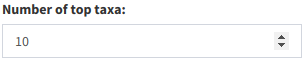
Top taxa number input
The "Subset taxa" tab allows the user to remove all species or OTUs belonging to a certain taxa. The user must choose a taxonomic rank in the dropdown list, then untick all taxa that they wish to see removed. Once they're done, tick 
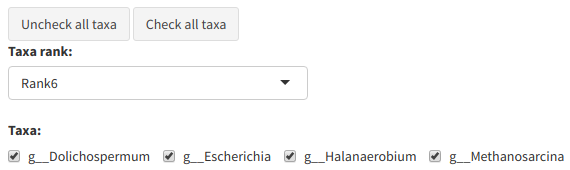
Example of the taxa subsetting menu
The user can remove individual samples from the dataset in the "Remove samples" tab. Like the previous section, to remove samples just untick all samples that should be removed and tick 
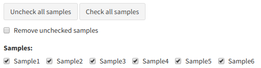
Remove samples menu example
It's possible to subset the plot by a value of prevalence - the ratio of OTU/species presence in samples. For example, a prevalence of 0.5 will make it so that any species that doesn't appear in at least 50% of samples will be removed from the dataset. In the "Prevalence [0-1]:" box, input a number between 0 and 1. Inputting a value of 1 will likely cause an error, unless there is an OTU that's present in 100% of samples.
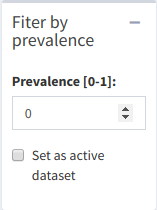
Prevalence subsetting menu
Displays a general summary of the entire dataset, based on the microbiome library's summarize_phyloseq() function. This includes smallest, largest and median reads, number of singletons, and whether the data is in compositional format or not.
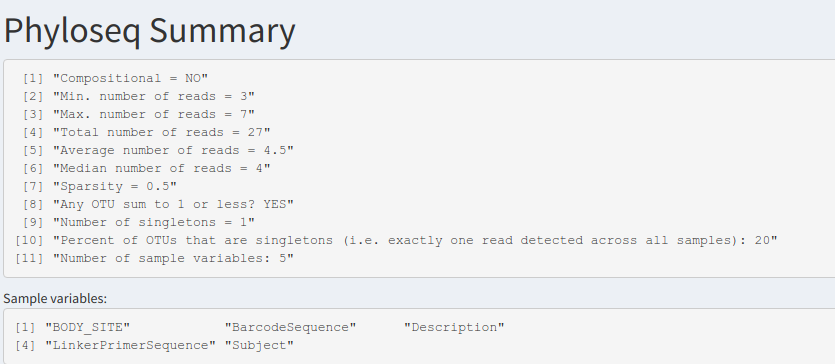
Phyloseq summary
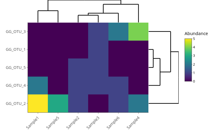
A heatmap that compares abundance values for each OTU on each sample.
Allows the user to view how abundant a given taxa is, generating abundance (absolute and relative) barplots which allow the samples to be sorted by metadata.
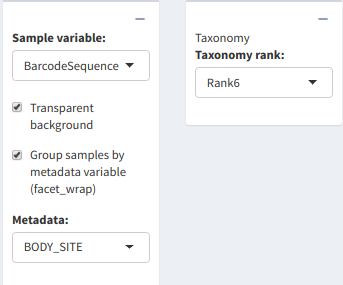
Plot generation menu
In the "Sample variable:" dropdown list, the user needs to pick the metadata variable which corresponds to the samples. If the uploaded dataset didn't have any metadata attached to it, the sample variable was automatically generated from the OTU table's sample headers.
By ticking 
The "Taxonomy Rank:" dropdown colors the bars based on the chosen taxonomic rank.
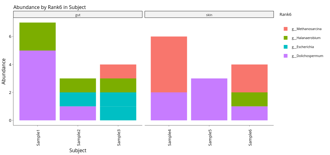
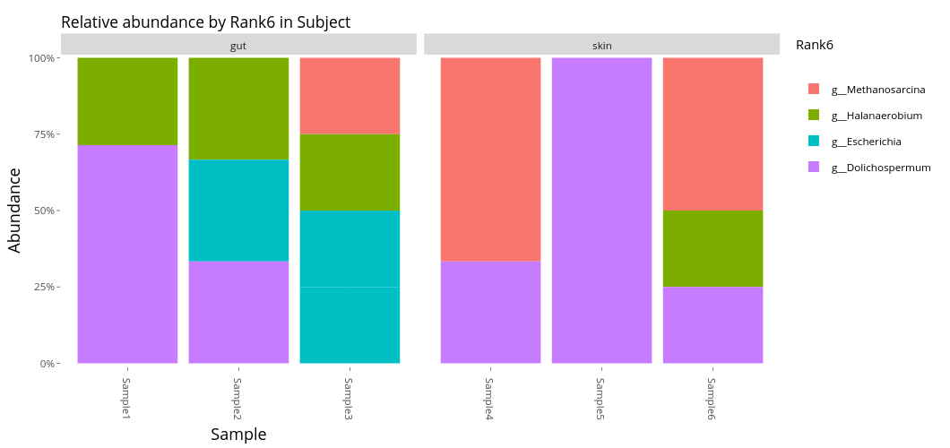
Absolute (top) and relative (bottom) abundance by Genus (Rank6), samples divided between gut and skin samples.
Alpha diversity is the index that measures diversity within a sample.
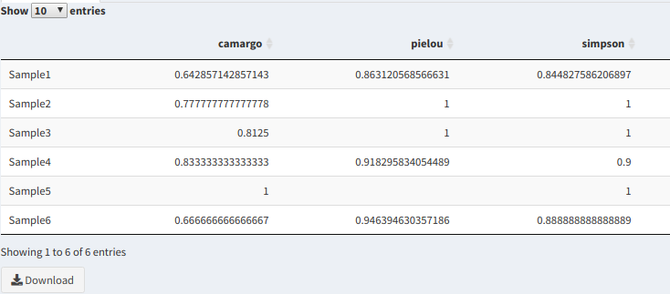
Biome-Shiny displays several tables with diversity measures in the samples, such as an Evenness Table (measures how equal the OTU numbers are in each sample), Abundance Table (measures the number of each OTU in the table, whether as a simple count or in relation to the full number of species in the sample) and a table with assorted diversity measures (measure richness, among other things).
Richness plot generation menu
Evenness table
The Richness Plot can be used to visualize these diversity measures. The "Samples:" dropdown list, much like in Community Composition, asks for the metadata variable corresponding to the dataset's samples. "Point color metadata" will give each point on the plot (corresponding to a sample) a color based on the chosen metadata variable.
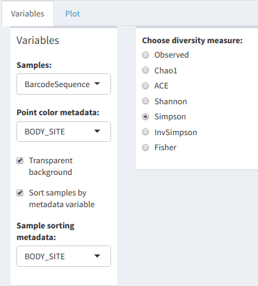
Richness table variables
Finally, it's possible to group samples by a metadata sample in the same way as the Community Composition plots.
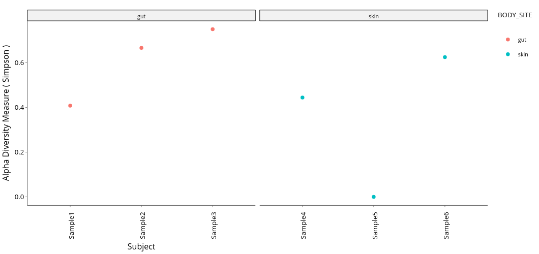
Richness plot example
Beta diversity is an index that measures diversity between samples. Biome-Shiny measures Beta diversity by the samples' general composition. This is done by generating a distance matrix and representing it as a PCA plot, where each point corresponds to a sample.
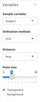
Distance PCA plot generation menu
The "Metadata:" dropdown list gives the points in the plot a color. There are a variety of ordination methods and distances to use, and not all ordination methods require distances. If in doubt, leave them on default settings.
Example PCA plot
The PERMANOVA test can be used to determine the importance of a sample variable in affecting the samples' composition. The test is applied over a user-input number of permutations, and with a dissimilarity index chosen by the user (default is "bray", though there are several more).
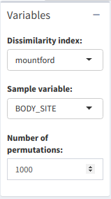
PERMANOVA test menu
The test's results can be viewed in a table, where a P-value between 0 and 1 determines the importance of the analyzed variable in affecting differences between samples
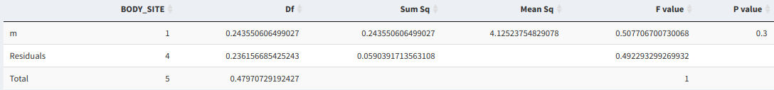
PERMANOVA results table
Visualization is done through a Top Factors plot, which applies the test in order to determine which OTUs are most important to differentiate samples in two different groups (i.e. given two different nationalities, which OTUs are more abundant in one nationality's sample group and which OTUs are more abundant in the other).
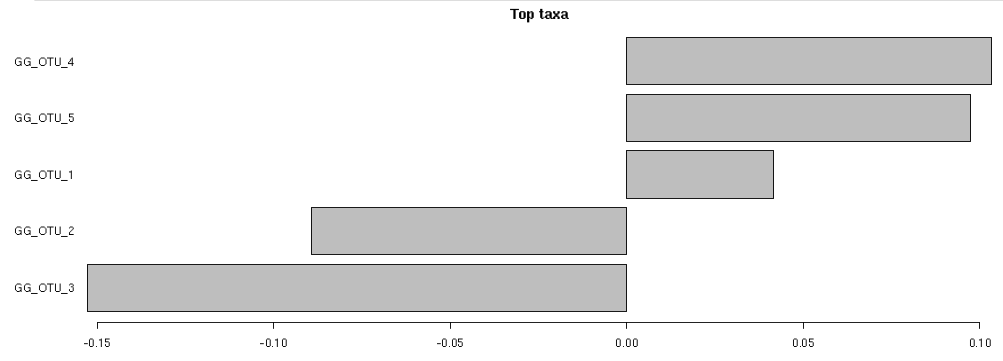
Top Factors plot
Individual tables and plots can be saved, either by pressing 

Alternatively, an HTML report can be downloaded by clicking 
-
Winston Chang, Joe Cheng, JJ Allaire, Yihui Xie and Jonathan McPherson (2019). shiny: Web Application Framework for R. R package version 1.4.0. https://CRAN.R-project.org/package=shiny
-
Winston Chang and Barbara Borges Ribeiro (2018). shinydashboard: Create Dashboards with 'Shiny'. R package version 0.7.1. https://CRAN.R-project.org/package=shinydashboard
-
Eric Bailey (2015). shinyBS: Twitter Bootstrap Components for Shiny. R package version 0.61. https://CRAN.R-project.org/package=shinyBS
-
Paul J. McMurdie and Joseph N Paulson (2019). biomformat: An interface package for the BIOM file format. https://github.com/joey711/biomformat/, http://biom-format.org/.
-
phyloseq: An R package for reproducible interactive analysis and graphics of microbiome census data. Paul J. McMurdie and Susan Holmes (2013) PLoS ONE 8(4):e61217.
-
Leo Lahti et al. microbiome R package. URL: http://microbiome.github.io
-
JJ Allaire and Yihui Xie and Jonathan McPherson and Javier Luraschi and Kevin Ushey and Aron Atkins and Hadley Wickham and Joe Cheng and Winston Chang and Richard Iannone (2019). rmarkdown: Dynamic Documents for R. R package version 1.18. URL https://rmarkdown.rstudio.com.
-
Yihui Xie, Joe Cheng and Xianying Tan (2019). DT: A Wrapper of the JavaScript Library 'DataTables'. R package version 0.10. https://CRAN.R-project.org/package=DT
-
H. Wickham. ggplot2: Elegant Graphics for Data Analysis. Springer-Verlag New York, 2016.
-
Alboukadel Kassambara (2019). ggpubr: 'ggplot2' Based Publication Ready Plots. R package version 0.2.4.999. https://rpkgs.datanovia.com/ggpubr/
-
Carson Sievert (2018) plotly for R. https://plotly-r.com
-
Tal Galili, Alan O'Callaghan, Jonathan Sidi, Carson Sievert; heatmaply: an R package for creating interactive cluster heatmaps for online publishing, Bioinformatics, , btx657, https://doi.org/10.1093/bioinformatics/btx657
-
Hadley Wickham (2017). tidyverse: Easily Install and Load the 'Tidyverse'. R package version 1.2.1. https://CRAN.R-project.org/package=tidyverse
-
Bob Rudis (2019). hrbrthemes: Additional Themes, Theme Components and Utilities for 'ggplot2'. R package version 0.6.0. https://CRAN.R-project.org/package=hrbrthemes
-
Hadley Wickham (2007). Reshaping Data with the reshape Package. Journal of Statistical Software, 21(12), 1-20. URL http://www.jstatsoft.org/v21/i12/.
-
Jari Oksanen, F. Guillaume Blanchet, Michael Friendly, Roeland Kindt, Pierre Legendre, Dan McGlinn, Peter R. Minchin, R. B. O'Hara, Gavin L. Simpson, Peter Solymos, M. Henry H. Stevens, Eduard Szoecs and Helene Wagner (2019). vegan: Community Ecology Package. R package version 2.5-6. https://CRAN.R-project.org/package=vegan
-
Erich Neuwirth (2014). RColorBrewer: ColorBrewer Palettes. R package version 1.1-2. https://CRAN.R-project.org/package=RColorBrewer
Biome-Shiny is licensed by Creative Commons Attribution 4.0 International. You are free to use, modify and distribute this software, under the condition that you attribute Biome-Shiny to BioData.pt and Henrique Costa.