35 Core Dynamic Programming Interview Questions

You can also find all 35 answers here 👉 Devinterview.io - Dynamic Programming

1. What is Dynamic Programming and how does it differ from recursion?

Dynamic Programming (DP) and recursion both offer ways to solve computational problems, but they operate differently.

Core Principles

• Recursion: Solves problems by reducing them to smaller, self-similar sub-problems, shortening the input until a base case is reached.
• DP: Breaks a problem into more manageable overlapping sub-problems, but solves each sub-problem only once and then stores its solution. This reduces the problem space and improves efficiency.

Key Distinctions

• Repetition: In contrast to simple recursion, DP uses memoization (top-down) or tabulation (bottom-up) to eliminate repeated computations.
• Directionality: DP works in a systematic, often iterative fashion, whereas recursive solutions can work top-down, bottom-up, or employ both strategies.

Example: Fibonacci Sequence

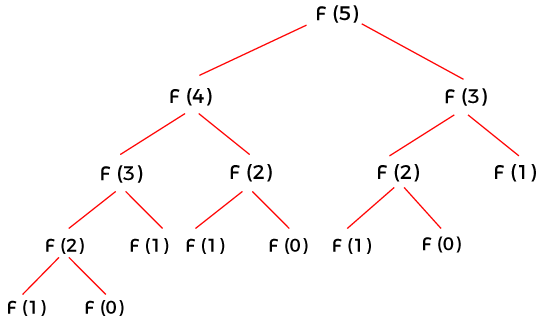
• Recursion: Directly calculates the $n$th number based on the $(n-1)$ and $(n-2)$ numbers. This results in many redundant calculations, leading to inefficient time complexity, often $O(2^n)$.

  def fibonacci_recursive(n):
      if n <= 1:
          return n
      return fibonacci_recursive(n-1) + fibonacci_recursive(n-2)
  

• DP:

  • Top-Down (using memoization): Caches the results of sub-problems, avoiding redundant calculations.

    def fibonacci_memoization(n, memo={}):
        if n <= 1:
            return n
        if n not in memo:
            memo[n] = fibonacci_memoization(n-1, memo) + fibonacci_memoization(n-2, memo)
        return memo[n]
    

  • Bottom-Up (using tabulation): Builds the solution space from the ground up, gradually solving smaller sub-problems until the final result is reached. It typically uses an array to store solutions.

    def fibonacci_tabulation(n):
        if n <= 1:
            return n
        fib = [0] * (n+1)
        fib[1] = 1
        for i in range(2, n+1):
            fib[i] = fib[i-1] + fib[i-2]
        return fib[n]
    

2. Can you explain the concept of overlapping subproblems?

Overlapping subproblems is a core principle of dynamic programming. It means that the same subproblem is encountered repeatedly during the execution of an algorithm. By caching previously computed solutions, dynamic programming avoids redundant computations, improving efficiency.

Visual Representation

In the grid above, each cell represents a subproblem. If the same subproblem (indicated by the red square) is encountered multiple times, it leads to inefficiencies as the same computation is carried out repeatedly.

In contrast, dynamic programming, by leveraging caching (the grayed-out cells), eliminates such redundancies and accelerates the solution process.

Real-World Examples

• Fibonacci Series: In $Fib(n) = Fib(n-1) + Fib(n-2)$, the recursive call structure entails repeated calculations of smaller fib values.

• Edit Distance:

  • For the strings "Saturday" and "Sunday", the subproblem of finding the edit distance between "Satur" and "Sun" is used in multiple paths of the decision tree for possible edits. This recurrence means the same subproblem of "Satur" to "Sun" will reoccur if it's not solved optimally in the initial step.

Code Example: Fibonacci

Here is the Python code:

# Simple Recursive Implementation
def fib_recursive(n):
    if n <= 1:
        return n
    return fib_recursive(n-1) + fib_recursive(n-2)

# Dynamic Programming using Memoization
def fib_memoization(n, memo={}):
    if n <= 1:
        return n
    if n not in memo:
        memo[n] = fib_memoization(n-1, memo) + fib_memoization(n-2, memo)
    return memo[n]

3. Define memoization and how it improves performance in Dynamic Programming.

Dynamic Programming often relies on two common strategies to achieve performance improvements - Tabulation and Memoization.

Memoization

Memoization involves storing calculated results of expensive function calls and reusing them when the same inputs occur again. This technique uses a top-down approach (starts with the main problem and breaks it down).

Advantages

• Enhanced Speed: Reduces redundant task execution, resulting in faster computational times.
• Code Simplicity: Makes code more readable by avoiding complex if-else checks and nested loops, improving maintainability.
• Resource Efficiency: Can save memory in certain scenarios by pruning the search space.
• Tailor-Made: Allows for customization of function calls, for instance, by specifying cache expiration.

Disadvantages

• Overhead: Maintaining a cache adds computational overhead.
• Scalability: In some highly concurrent applications or systems with heavy memory usage, excessive caching can lead to caching problems and reduced performance.
• Complexity: Implementing memoization might introduce complexities, such as handling cache invalidation.

Example: Fibonacci Series

Without memoization, a recursive Fibonacci function has an exponential time complexity of $\mathcal{O}(2^n)$. Implementing memoization reduces the time complexity to $\mathcal{O}(n)$.

Python Code

Here is the Python code:

from functools import lru_cache

@lru_cache(maxsize=None)  # Optional for memoization using cache decorator
def fibonacci(n):
    if n <= 1:
        return n
    return fibonacci(n-1) + fibonacci(n-2)
 

4. What is the difference between top-down and bottom-up approaches in Dynamic Programming?

When employing dynamic programming, you have a choice between top-down and bottom-up approaches. Both strategies aim to optimize computational resources and improve running time, but they do so in slightly different ways.

Top-Down (Memoization)

Top-down, also known as memoization, involves breaking down a problem into smaller subproblems and then solving them in a top-to-bottom manner. Results of subproblems are typically stored for reuse, avoiding redundancy in calculations and leading to better efficiency.

Example: Fibonacci Sequence

In the top-down approach, we calculate $fib(n-1)$ and $fib(n-2)$ before combining the results to yield $fib(n)$. This typically involves the use of recursive functions and a lookup table to store previously computed values.

def fib_memo(n, memo={}):
    if n in memo:
        return memo[n]
    if n <= 2:
        return 1
    memo[n] = fib_memo(n-1, memo) + fib_memo(n-2, memo)
    return memo[n]

Bottom-Up (Tabulation)

The bottom-up method, also referred to as tabulation, approaches the problem from the opposite direction. It starts by solving the smallest subproblem and builds its way up to the larger one, without needing recursion.

Example: Fibonacci Sequence

For the Fibonacci sequence, we can compute the values iteratively, starting from the base case of 1 and 2.

def fib_tabulate(n):
    if n <= 2:
        return 1
    fib_table = [0] * (n + 1)
    fib_table[1] = fib_table[2] = 1
    for i in range(3, n + 1):
        fib_table[i] = fib_table[i-1] + fib_table[i-2]
    return fib_table[n]

This approach doesn't incur the overhead associated with function calls and is often more direct and therefore faster. Opting for top-down or bottom-up DP, though, depends on the specifics of the problem and the programmer's preferred style.

5. Explain the importance of state definition in Dynamic Programming solutions.

State definition serves as a crucial foundation for Dynamic Programming (DP) solutions. It partitions the problem into overlapping subproblems and enables both top-down (memoization) and bottom-up (tabulation) techniques for efficiency.

Why State Definition Matters in DP

• Subproblem Identification: Clearly-defined states help break down the problem, exposing its recursive nature.

• State Transition Clarity: Well-structured state transitions make the problem easier to understand and manage.

• Memory Efficiency: Understanding the minimal information needed to compute a state avoids unnecessary memory consumption or computations.

• Code Clarity: Defined states result in clean and modular code.

Categorization of DP Problems

1. Optimization Problems

Problems aim to maximize or minimize a particular value. They often follow a functional paradigm, where each state is associated with a value.

Example: Finding the longest increasing subsequence in an array.

2. Counting Problems

These problems require counting the number of ways to achieve a certain state or target. They are characterized by a combinatorial paradigm.

Example: Counting the number of ways to make change for a given amount using a set of coins.

3. Decision-Making Problems

The objective here is more about whether a solution exists or not rather than quantifying it. This kind of problem often has a binary nature—either a target state is achievable, or it isn't.

Example: Determining whether a given string is an interleaving of two other strings.

Unified by their dependence on overlapping subproblems and optimal substructure, these problem types benefit from a state-based approach, laying a foundation for efficient DP solutions.

6. Compute the Fibonacci sequence using Dynamic Programming.

Problem Statement

The task is to compute the Fibonacci sequence using dynamic programming, in order to reduce the time complexity from exponential to linear.

Solution

Using Tabulation

Tabulation, also known as the bottom-up method, is an iterative approach. It stores and reuses the results of previous subproblems in a table.

Algorithm Steps

1. Initialize an array, fib[], with base values.
2. For $i = 2$ to $n$, compute fib[i] using the sum of the two previous elements in fib[].

Complexity Analysis

• Time Complexity: $O(n)$. This is an improvement over the exponential time complexity of the naive recursive method.
• Space Complexity: $O(n)$, which is primarily due to the storage needed for the fib[] array.

Implementation

Here is the Python code:

def fibonacci_tabulation(n):
    if n <= 1:
        return n
    
    fib = [0] * (n + 1)
    fib[1] = 1

    for i in range(2, n + 1):
        fib[i] = fib[i-1] + fib[i-2]

    return fib[n]

7. Implement a solution to the Coin Change Problem using DP.

Problem Statement

The coin change problem is an optimization task often used as an introduction to dynamic programming. Given an array of coins and a target amount, the goal is to find the minimum number of coins needed to make up that amount. Each coin can be used an unlimited number of times, and an unlimited supply of coins is assumed.

Example: With coins [1, 2, 5] and a target of 11, the minimum number of coins needed is via the combination 5 + 5 + 1 (3 coins).

Solution

The optimal way to solve the coin change problem is through dynamic programming, specifically using the bottom-up approach.

By systematically considering smaller sub-problems first, this method allows you to build up the solution step by step and avoid redundant calculations.

Algorithm Steps

1. Create an array dp of size amount+ 1 and initialize it with a value larger than the target amount, for instance, amount + 1.
2. Set dp[0] = 0, indicating that zero coins are needed to make up an amount of zero.
3. For each i from 1 to amount and each coin:
   • If coin is less than or equal to i, compute dp[i] as the minimum of its current value and 1 + dp[i - coin]. The 1 represents using one of the coin denomination, and dp[i - coin] represents the minimum number of coins needed to make up the remaining amount.
4. The value of dp[amount] reflects the minimum number of coins needed to reach the target, given the provided denominations.

Complexity Analysis

• Time Complexity: $O(\text{{amount}} \times \text{{len(coins)}})$. This arises from the double loop structure.
• Space Complexity: $O(\text{{amount}})$. This is due to the dp array.

Implementation

Here is the Python code:

def coinChange(coins, amount):
    dp = [amount + 1] * (amount + 1)
    dp[0] = 0

    for i in range(1, amount + 1):
        for coin in coins:
            if coin <= i:
                dp[i] = min(dp[i], 1 + dp[i - coin])

    return dp[amount] if dp[amount] <= amount else -1

8. Use Dynamic Programming approach to solve the 0/1 Knapsack problem.

Problem Statement

Consider a scenario where a thief is confronted with $n$ items; each has a weight, $w_i$, and a value, $v_i$. The thief has a knapsack that can only hold a certain weight, noted as $W$. The task is to determine the combination of items that the thief should take to ensure the best value without surpassing the weight limit.

Solution

This programming challenge can be effectively handled using dynamic programming (DP). The standard, and most efficient, version of this method is based on an approach known as the table-filling.

Steps

1. Creating the 2D Table: A table of size $(n + 1) \times (W + 1)$ is established. Each cell represents the optimal value for a specific combination of items and knapsack capacities. Initially, all cells are set to 0.

2. Filling the Table: Starting from the first row (representing 0 items), each subsequent row is determined based on the previous row's status.

   $\cdot$ For each item, and for each possible knapsack weight (for i, w in enumerate(weights)), the DP algorithm decides whether adding the item would be more profitable.

   $\cdot$ The decision is made by comparing the value of the current item plus the best value achievable with the remaining weight and items (taken from the previous row), versus the best value achieved based on the items up to this point but without adding the current item.

3. Deriving the Solution: Once the entire table is filled, the optimal set of items is extracted by backtracking through the table, starting from the bottom-right cell.

Complexity Analysis

• Time Complexity: $O(n \cdot W)$ where $n$ is the number of items and $W$ is the maximum knapsack capacity.
• Space Complexity: $O(n \cdot W)$ due to the table.

Implementation

Here is the Python code:

def knapsack(weights, values, W):
    n = len(weights)
    dp = [[0 for _ in range(W + 1)] for _ in range(n + 1)]

    for i in range(1, n + 1):
        for w in range(1, W + 1):
            if weights[i-1] > w:
                dp[i][w] = dp[i-1][w]
            else:
                dp[i][w] = max(dp[i-1][w], values[i-1] + dp[i-1][w-weights[i-1]])

    # Backtrack to get the selected items
    selected_items = []
    i, w = n, W
    while i > 0 and w > 0:
        if dp[i][w] != dp[i-1][w]:
            selected_items.append(i-1)
            w -= weights[i-1]
        i -= 1

    return dp[n][W], selected_items

Dynamic Programming Optimization

While the above solution is straightforward, it uses $O(n \cdot W)$ space. This can be reduced to $O(W)$ through an optimization known as space-compression or roll-over technique.

9. Implement an algorithm for computing the longest common subsequence of two sequences.

Problem Statement

The task is to find the Longest Common Subsequence (LCS) of two sequences, which can be any string, including DNA strands.

For instance, given two sequences, ABCBDAB and BDCAB, the LCS would be BCAB.

Solution

The optimal substructure and overlapping subproblems properties make it a perfect problem for Dynamic Programming.

1. Basic Idea

We start with two pointers at the beginning of each sequence. If the characters match, we include them in the LCS and advance both pointers. If they don't, we advance just one pointer and repeat the process. We continue until reaching the end of at least one sequence.

2. Building the Matrix

• Initialize a matrix L[m+1][n+1] with all zeros, where m and n are the lengths of the two sequences.
• Traverse the sequences. If X[i] == Y[j], set L[i+1][j+1] = L[i][j] + 1. If not, set L[i+1][j+1] to the maximum of L[i][j+1] and L[i+1][j].
• Start from L[m][n] and backtrack using the rules based on which neighboring cell provides the maximum value, until i or j becomes 0.

3. Complexity Analysis

• Time Complexity: $O(mn)$, where $m$ and $n$ are the lengths of the two sequences. This is due to the nested loop used to fill the matrix.
• Space Complexity: $O(mn)$, where $m$ and $n$ are the lengths of the two sequences. This is associated with the space used by the matrix.

Implementation

Here is the Python code:

def lcs(X, Y):
    m, n = len(X), len(Y)
    # Initialize the matrix with zeros
    L = [[0] * (n + 1) for _ in range(m + 1)]

    # Building the matrix
    for i in range(m):
        for j in range(n):
            if X[i] == Y[j]:
                L[i + 1][j + 1] = L[i][j] + 1
            else:
                L[i + 1][j + 1] = max(L[i + 1][j], L[i][j + 1])

    # Backtrack to find the LCS
    i, j = m, n
    lcs_sequence = []
    while i > 0 and j > 0:
        if X[i - 1] == Y[j - 1]:
            lcs_sequence.append(X[i - 1])
            i, j = i - 1, j - 1
        elif L[i - 1][j] > L[i][j - 1]:
            i -= 1
        else:
            j -= 1

    return ''.join(reversed(lcs_sequence))

# Example usage
X = "ABCBDAB"
Y = "BDCAB"
print("LCS of", X, "and", Y, "is", lcs(X, Y))

10. Solve matrix chain multiplication problem with Dynamic Programming.

Problem Statement

Given a sequence of matrices $A_1, A_2, \ldots, A_n$, the matrix chain multiplication problem is to find the most efficient way to multiply these matrices.

The goal is to minimize the number of scalar multiplications, which is dependent on the order of multiplication.

Solution

The most optimized way to solve the Matrix Chain Multiplication problem uses Dynamic Programming (DP).

Algorithm Steps

1. Subproblem Definition: For each $i, j$ pair (where $1 \leq i \leq j \leq n$), we find the optimal break in the subsequence $A_i \ldots A_j$. Let the split be at $k$, such that the cost of multiplying the resulting A matrix chain using the split is minimized.

2. Base Case: The cost is 0 for a single matrix.

3. Build Up: For a chain of length $l$, iterate through all $i, j, k$ combinations and find the one with the minimum cost.

4. Optimal Solution: The DP table helps trace back the actual parenthesization and the optimal cost.

Key Insight: Optimal parenthesization for a chain involves an optimal split.

Complexity Analysis

• Time Complexity: $O(n^3)$ - Three nested loops for each subchain length.
• Space Complexity: $O(n^2)$ - DP table.

Illustrative Python Code

import sys

def matrix_chain_order(p):
    n = len(p) - 1    # Number of matrices
    m = [[0 for _ in range(n)] for _ in range(n)]  # Cost table
    s = [[0 for _ in range(n)] for _ in range(n)]  # Splitting table

    for l in range(2, n+1):  # l is the chain length
        for i in range(n - l + 1):
            j = i + l - 1
            m[i][j] = sys.maxsize
            for k in range(i, j):
                q = m[i][k] + m[k+1][j] + p[i]*p[k+1]*p[j+1]
                if q < m[i][j]:
                    m[i][j] = q
                    s[i][j] = k

    return m, s

11. What are the trade-offs between memoization and tabulation in Dynamic Programming?

While both memoization and tabulation optimize dynamic programming algorithms for efficiency, they differ in their approaches and application.

Memoization

• Divide and Conquer Technique: Breaking a problem down into smaller, more manageable sub-problems.

• Approach: Top-down, meaning you start by solving the main problem and then compute the sub-problems as needed.

• Key Advantage: Eliminates redundant calculations, improving efficiency.

• Potential Drawbacks:

  • Can introduce overhead due to recursion.
  • Maintaining the call stack can consume significant memory, especially in problems with deep recursion.

Tabulation

• Divide and Conquer Technique: Breaks a problem down into smaller, more manageable sub-problems.

• Approach: Bottom-up, which means you solve all sub-problems before tackling the main problem.

• Key Advantage: Operates without recursion, avoiding its overhead and limitations.

• Potential Drawbacks:

  • Can be less intuitive to implement, especially for problems with complex dependencies.
  • May calculate more values than required for the main problem, especially if its size is significantly smaller than the problem's domain.

12. How do you determine the time complexity of a Dynamic Programming algorithm?

Dynamic Programming (DP) aims to solve problems by breaking them down into simpler subproblems. However, tracking the time complexity of these approaches isn't always straightforward because the time complexity can vary between algorithms and implementations.

Common DP Patterns and Their Time Complexity

• Top-Down with Memoization:

  • Time Complexity: Usually, it aligns with the Top-Down (1D/2D array) method being the slowest but can't be generalized.
  • Historically, it might be $O(2^n)$, and upon adding state space reduction techniques, it typically reduces to $O(nm)$, where $n$ and $m$ are the state space parameters. However, modern implementations like the A* algorithm or RL algorithms can offer a flexible time complexity.
  • Space Complexity: $O(\text{State Space})$

• Bottom-Up with 1D Array:

  • Time Complexity: Often $O(n \cdot \text{Subproblem Complexity})$.
  • Space Complexity: $O(1)$ or $O(n)$ with memoization.

• Bottom-Up with 2D Array:

  • Time Complexity: Generally $O(mn \cdot \text{Subproblem Complexity})$, where $m$ and $n$ are the 2D dimensions.
  • Space Complexity: $O(mn)$

• State Space Reduction Techniques:

  • Techniques like Sliding Window, Backward Induction, and Cycle Breaking reduce the state space or the size of the table, ultimately influencing both time and space complexity metrics.

Code Example: Fibonacci Sequence

Here is the Python code:

def fib_top_down(n, memo):
    if n <= 1:
        return n
    if memo[n] is None:
        memo[n] = fib_top_down(n-1, memo) + fib_top_down(n-2, memo)
    return memo[n]

def fib_bottom_up(n):
    if n <= 1:
        return n
    prev, current = 0, 1
    for _ in range(2, n+1):
        prev, current = current, prev + current
    return current

13. Describe techniques to optimize space complexity in Dynamic Programming problems.

Dynamic Programming (DP) can be memory-intensive due to its tabular approach. However, there are several methods to reduce space complexity.

Techniques to Reduce Space Complexity in DP

1. Tabular-vs-Recursive Methods: Use tabular methods for bottom-up DP and minimize space by only storing current and previous states if applicable.

2. Divide-and-Conquer: Optimize top-down DP with a divide-and-conquer approach.

3. Interleaved Computation: Reduce space needs by computing rows or columns of a table alternately.

4. High-Level Dependency: Represent relationships between subproblems to save space, as seen in tasks like edit distance and 0-1 Knapsack.

5. Stateful Compression: For state machines or techniques like Rabin-Karp, compact the state space using a bitset or other memory-saving structures.

6. Locational Memoization: In mazes and similar problems, memoize decisions based on present position rather than the actual state of the system.

7. Parametric Memory: For problems such as the egg-dropping puzzle, keep track of the number of remaining parameters.

14. What is state transition, and how do you derive state transition relations?

State transition relations describe how a problem's state progresses during computation. They are a fundamental concept in dynamic programming, used to define state transitions in the context of a mathematical model and its computational representation.

Modeling State Transitions

1. State Definition: Identify the core components that define the state of the problem. This step requires a deep understanding of the problem and the information necessary to model the state accurately. State may be defined flexibly, depending on the problem's complexity and nuances.

2. State Transitions: Define how the state evolves over time or through an action sequence. Transition functions or relations encapsulate the possible state changes, predicated on specific decisions or actions.

3. Initial State: Establish the starting point of the problem. This step is crucial for state-based algorithms, ensuring that the initial configuration aligns with practical requirements.

4. Terminal State Recognition: Determine the criteria for identifying when the state reaches a conclusion or a halting condition. For dynamic programming scenarios, reaching an optimal or final state can trigger termimnation or backtracking.

State Transition's Computational Role

• Memory Mechanism: It allows dynamic programming to store and reuse state information, avoiding redundant calculations. This capacity for efficient information retention differentiates it from more regular iterative algorithms.
• Information Representation: State spaces and their transitions capture essential information about various problem configurations and their mutual relationships.

Dynamic programming accomplishes a balance between thoroughness and computational efficiency by leveraging the inherent structure of problems.

Code Example: Knapsack Problem & State Transitions

Here is the Python code:

def knapsack01(values, weights, capacity):
    n = len(values)
    dp = [[0 for _ in range(capacity + 1)] for _ in range(n + 1)]

    for i in range(1, n + 1):
        for w in range(1, capacity + 1):
            if weights[i - 1] <= w:
                dp[i][w] = max(values[i - 1] + dp[i - 1][w - weights[i - 1]], dp[i - 1][w])
            else:
                dp[i][w] = dp[i - 1][w]

    return dp[n][capacity], dp

values = [60, 100, 120]
weights = [10, 20, 30]
capacity = 50
max_value, state_table = knapsack01(values, weights, capacity)
print(f"Maximum value achievable: {max_value}")

15. Find the longest palindromic substring in a given string.

Problem Statement

Find the longest palindromic substring within a string s.

• Input: "babad"
• Output: "bab" or "aba" — The two substrings "bab" and "aba" are both valid solutions.

Solution

The problem can be solved using either an Expand Around Center algorithm or Dynamic Programming. Here, I will focus on the more efficient dynamic programming solution.

Dynamic Programming Algorithm Steps

1. Define a 2D table, dp, where dp[i][j] indicates whether the substring from index i to j is a palindrome.
2. Initialize the base cases: single characters are always palindromes, and for any two adjacent characters, they form a palindrome if they are the same character.
3. Traverse the table diagonally, filling it from shorter strings to longer ones since the state of a longer string depends on the states of its shorter substrings.

Complexity Analysis

• Time Complexity: $O(n^2)$
• Space Complexity: $O(n^2)$

Implementation

Here is the Python code:

def longestPalindrome(s: str) -> str:
    n = len(s)
    if n < 2 or s == s[::-1]:
        return s

    start, maxlen = 0, 1
    # Initialize dp table. dp[i][i] is always True (single character).
    dp = [[False] * n for _ in range(n)]
    for i in range(n):
        dp[i][i] = True

    for j in range(1, n):
        for i in range(j):
            # Check for palindrome while updating dp table.
            if s[i] == s[j] and (dp[i+1][j-1] or j - i <= 2):
                dp[i][j] = True
                # Update the longest palindrome found so far.
                if j - i + 1 > maxlen:
                    start, maxlen = i, j - i + 1

    return s[start : start + maxlen]

# Test the function
print(longestPalindrome("babad"))  # Output: "bab"

Explore all 35 answers here 👉 Devinterview.io - Dynamic Programming