50 Fundamental Gradient Descent Interview Questions

You can also find all 50 answers here 👉 Devinterview.io - Gradient Descent

1. What is gradient descent?

Gradient descent is a fundamental optimization technique within machine learning and other fields. It was introduced by the physicist Peter Molnar in 1964 and later independently rediscovered by other researchers.

Intuition

The basic idea of gradient descent is to iteratively update model parameters in the direction that minimizes a performance metric, often represented by a cost function or loss function.

Mathematically, this process is characterized by the gradient of the cost function, computed using backpropagation in the case of neural networks.

Formulation

Let $J(\boldsymbol{\theta})$ be the cost function and $\boldsymbol{\theta}$ be the parameter vector.

The update rule for each parameter can be expressed as:

$$ \theta_j := \theta_j - \alpha \frac{\partial J(\boldsymbol{\theta})}{\partial \theta_j} $$

Here, $\alpha$ is the learning rate and $\frac{\partial J(\boldsymbol{\theta})}{\partial \theta_j}$ is the partial derivative of the cost function with respect to the parameter $\theta_j$.

Visual Analogy

One can visualize gradient descent as a person trying to find the bottom of a valley (the cost function).

The individual takes small steps downhill (representing parameter updates), guided by the slope (the gradient) and the step size $\alpha$.

Mode of Operation

• Batch Gradient Descent: Computes the gradient for the entire dataset and takes a step. This can be slow for large datasets due to its high computational cost.

• Stochastic Gradient Descent (SGD): Computes the gradient for each data point and takes a step. It's faster but more noisy.

• Mini-batch Gradient Descent: Computes the gradient for small batches of data, offering a compromise between batch and stochastic methods.

Considerations

Learning Rate

Selecting an appropriate learning rate is crucial.

• If it's too large, overshoot may occur, and the algorithm could fail to converge.
• If it's too small, the algorithm might be slow or get trapped in local minima.

Convergence

Stopping criteria, such as a predefined number of iterations or a threshold for the change in the cost function, are employed to determine when the algorithm has converged.

Local Minima

While gradient descent provides no guarantee of finding the global minimum, in practice, it often suffices to reach a local minimum.

Code Example: Batch Gradient Descent

Here is the Python code:

def batch_gradient_descent(X, y, theta, alpha, iterations):
    m = len(y)  # Number of training examples
    
    for _ in range(iterations):
        error = X.dot(theta) - y  # Compute the error
        gradient = X.T.dot(error) / m  # Compute the gradient
        theta -= alpha * gradient  # Update parameters
    
    return theta

Beyond the Basics

• Momentum: Incorporates the running average of past gradients to accelerate convergence in the relevant directions.
• Adaptive Learning Rates: Algorithms like AdaGrad, RMSProp, and Adam adjust learning rates adaptively for each parameter.
• Beyond the Gradient: Evolutionary algorithms, variational methods, and black-box optimization techniques are avenues for optimization beyond the gradient.

2. What are the main variants of gradient descent algorithms?

Gradient Descent comes in several variants, each with its unique way of updating model parameters.

Common Variants of Gradient Descent

Stochastic Gradient Descent (SGD)

• Update method: Utilizes a single random training example for updating parameters.
• Benefits: Faster computations; useful when data is abundant and diverse.

    def sgd_step(learning_rate, model, data):
        random_example = random.choice(data)
        gradient = compute_gradient(model, random_example)
        model.parameters -= learning_rate * gradient

Mini-batch Gradient Descent

• Update method: Strikes a balance between full-batch and stochastic, using a small, fixed number of examples for each parameter update.
• Benefits: Computationally efficient and statistically more stable than SGD.

    def mini_batch_step(learning_rate, model, data, batch_size):
        batch = random.sample(data, batch_size)
        gradient = average([compute_gradient(model, example) for example in batch])
        model.parameters -= learning_rate * gradient

Momentum

• Update method: Uses a rolling average of gradients to update parameters, which can accelerate convergence and overcome local minima.
• Benefits: Effective in speeding up training on noisy or high-dimensional data.

    def momentum_step(learning_rate, model, data, gamma, prev_velocity):
        gradient = compute_gradient(model, data)
        velocity = gamma * prev_velocity + learning_rate * gradient
        model.parameters -= velocity
        return velocity

RMSprop (Root Mean Square Propagation)

• Update method: Adapts learning rates by dividing the gradient by a running average of its recent magnitudes.
• Benefits: Tends to converge more quickly than GD and can be less sensitive to learning rate hyperparameters.

    def rmsprop_step(learning_rate, model, data, epsilon, running_avg, gradient_sq):
        gradient = compute_gradient(model, data)
        running_avg = running_avg * 0.9 + (1 - 0.9) * gradient
        model.parameters -= learning_rate * gradient / np.sqrt(running_avg + epsilon)
        return running_avg

Adam (Adaptive Moment Estimation)

• Update method: Combines momentum and RMSprop, using first and second moment estimations of gradients to adapt learning rates.
• Benefits: Often performs well across different types of datasets.

    def adam_step(t, learning_rate, model, data, beta1, beta2, m, v):
        gradient = compute_gradient(model, data)
        m = beta1 * m + (1 - beta1) * gradient
        v = beta2 * v + (1 - beta2) * gradient ** 2
        m_hat = m / (1 - beta1 ** t)
        v_hat = v / (1 - beta2 ** t)
        model.parameters -= learning_rate * m_hat / (np.sqrt(v_hat) + 1e-8)
        return m, v

3. Explain the importance of the learning rate in gradient descent.

Learning rate plays a pivotal role in controlling the rate and accuracy of optimization during gradient descent. Essentially, it determines the step size for each iteration, allowing the algorithm to reach the minima more efficiently.

Key Concepts

Convergence

• A moderate learning rate ensures gradient descent convergence to the nearest local optima or global optima.

• If the learning rate is too small, the algorithm might need an excessive number of iterations to converge. Conversely, an excessively high learning rate might cause the algorithm to overshoot or oscillate around the minima, leading to non-convergence.

Efficiency and Accuracy

• A larger learning rate results in a faster reach to the minima, but this might cause the optimization process to be less accurate.

• A smaller learning rate can yield higher accuracy, but it might necessitate a longer computation time.

Contextual Flexibility

• Adaptive learning rates, such as those used in stochastic gradient descent or variants like Adagrad, RMSprop, and Adam, adapt the learning rate during training.

• Mini-batch gradient descent, which typically combines a fixed learning rate with stochastic steps, has introduced a more dynamic approach to learning rate determination.

Practical Considerations

1. Model Complexity: More complex models, or those with a high degree of multicollinearity, might necessitate careful tuning of the learning rate.

2. Data Variability: Datasets with varying scales across features might require learning rate adaptation.

3. Time and Resource Constraints: The choice of learning rate also impacts the computational time required for training. Validating and adjusting the learning rate could consume additional resources.

Automated Learning Rate Selection

Emerging techniques, such as hyperparameter tuning and grid search or random search, have simplified the process of learning rate selection. These methods can automatically determine the ideal learning rate or a range of learning rates based on the underlying model, dataset, and optimization task.

Consider the following Python example using the Keras library and its callbacks module:

import tensorflow as tf
from tensorflow.keras.callbacks import ReduceLROnPlateau

# Define the optimizer
optimizer = tf.keras.optimizers.SGD(learning_rate=0.1)

# Define the learning rate reduction callback
lr_reduce = ReduceLROnPlateau(monitor='val_loss', factor=0.5, patience=5, min_lr=0.001)

# Compile the model
model.compile(optimizer=optimizer, loss='mse', metrics=['mae'])

# Train the model using the learning rate reduction callback
model.fit(X_train, y_train, epochs=100, callbacks=[lr_reduce], validation_data=(X_val, y_val))

4. How does gradient descent help in finding the local minimum of a function?

Gradient descent is an iterative optimization algorithm that minimizes a differentiable function. It's especially useful in machine learning for minimizing cost or error functions.

Mechanism of Gradient Descent for Minimization

1. Starting Point Selection: The algorithm begins at a chosen point, called the initial guess or starting point.

2. Iteration: At each step $i$, gradient descent updates the current point by subtracting a fraction of the negative gradient.

$$ \text{New point} = \text{Old point} - \eta_i \cdot \nabla f(\text{Old point}) $$

The symbol $\eta_i$ represents the learning rate at step $i$.

3. Convergence: The algorithm stops when certain criteria are met, such as reaching a preset number of steps, the magnitude of the gradient becoming small, or small change in the cost function between iterations.

4. Optimized Point: The final point, if the algorithm converges, is an optimized solution that minimizes the objective function within a particular range.

Mathematics Behind Gradient Descent

The method follows the intuition that a point is a potential local minimum if moving in the opposite direction of the gradient reduces the function value.

For a function $f$ with a single variable, the update rule is given by:

$$ x_{k+1} = x_k - \eta \cdot f'(x_k) $$

where $f'(x)$ is the first derivative of $f$ evaluated at $x$ and $\eta$ is the learning rate.

The same concept extends to functions of multiple variables. The update rule for a point $\mathbf{x} = (x_1, x_2, \ldots, x_n)$ is:

$$ \mathbf{x}_{k+1} = \mathbf{x}_k - \eta \cdot \nabla f(\mathbf{x}_k) $$

Here, $\nabla f(\mathbf{x})$ is the gradient vector of $f$ evaluated at $\mathbf{x}$, and $\eta$ is the learning rate.

5. What challenges arise when using gradient descent on non-convex functions?

Gradient Descent can face several issues when dealing with non-convex functions.

Challenges of using Gradient Descent on Non-Convex Functions

1. Local Minima: Gradient Descent is prone to getting stuck in local minima in non-convex functions.

2. Saddle Points: These points have zero gradients but are not optima. Gradient Descent can linger around saddle points, slowing convergence.

3. Vanishing Gradient: The gradients near the minimum can become extremely small, causing slow learning or stagnation.

4. Chaotic Optimization Paths: Non-convex functions might have regions where the loss landscape is chaotic, leading to erratic optimization paths.

5. Overshooting: Distant jump locations due to large gradients might lead the algorithm away from minima, making it hard to converge.

6. Initial Point Sensitivity: Convergence might depend heavily on the starting point, leading to varied results across different initializations.

7. Plateaus and Flat Regions: Extensive flat regions can decelerate optimization by stalling gradient-descent updates.

8. Cliffs and Ridges: Steep, narrow cliffs or ridges can misguide optimization by pushing the algorithm off-course.

6. Explain the purpose of using gradient descent in machine learning models.

In the context of machine learning, specifically in learning algorithms or neural networks, the main reason we use gradient descent is the process of iteratively reducing losses: it helps to reach the optimal solution without having to compute a precise gradient at each iteration.

Core Principle: Minimizing Loss

The ultimate goal of a learning algorithm is to minimize a chosen loss function, also known as the cost or objective function. This function assesses the performance of the model by comparing its predictions to the actual data.

By reducing the loss function, we enhance the model's capability to make accurate predictions.

Challenge: Loss Minimization in High Dimensions

In practice, models often have numerous parameters, leading to high-dimensional spaces. Minimizing the loss function poses a formidable challenge in such multi-dimensional domains.

Limitation: Direct Computation of Minima is Not Viable

In multi-dimensional settings, calculating the analytical form of the minima is often unfeasible since it requires solving partial differential equations for high-dimensional spaces. This complexity makes direct computation impractical.

Approach: Step by Step Error Reduction

Gradient descent overcomes this predicament by approaching the minima in a stepwise manner. It continually updates the model parameters based on the observed error, thereby minimizing the loss function.

At each iteration, the algorithm 'follows the slope' by moving in the direction that shows the most rapid decrease in the cost function.

Practical Steps

1. Initializing Model Parameters: Begin by setting the model's parameters randomly or with specific initialization techniques.

2. Computing the Loss Gradient: Evaluate the gradient of the loss function with respect to the model parameters. This step identifies the direction of maximum increase in the loss function.

3. Updating the Parameters: Adjust the current parameter values in the direction opposite to the gradient, leading to a reduction in the loss.

   The update rule for each parameter, denoted as $\theta_i$, can be expressed as:

$$ \theta_i \leftarrow \theta_i - \alpha \cdot \text{gradient}_i $$

where $\alpha$ is the learning rate, a small positive value that controls the step size.

4. Repeating Iterations: This process continues for a set number of iterations or until the improvement in the loss function falls below a specified threshold.

Algorithm Variants for Different Data Types

• Batch Gradient Descent: Utilizes the entire dataset for each iteration. This method is computationally intensive and might be slow in the context of big data.

• Stochastic Gradient Descent (SGD): Uses a single randomly selected data point to compute the gradient and update the model parameters. Although this method is more random, it's computationally efficient, especially when dealing with large datasets.

• Mini-Batch Gradient Descent: A blend of both batch and stochastic gradient descent. It uses a small, fixed number of data points for each iteration. This method combines the advantages of the other two methods: it's computationally efficient and less prone to random fluctuations.

Practical Considerations

• Learning Rate: The step size in the direction of the negative gradient. Selecting an appropriate learning rate is crucial for the convergence and stability of the algorithm.

• Convergence: An effective gradient descent algorithm should converge to an optimal solution. This might involve monitoring the change in the loss function across iterations.

• Model Initialization: As the performance of gradient descent can be sensitive to the starting point, techniques like Xavier and Glorot initialization are often used to set initial values.

Visual Representation

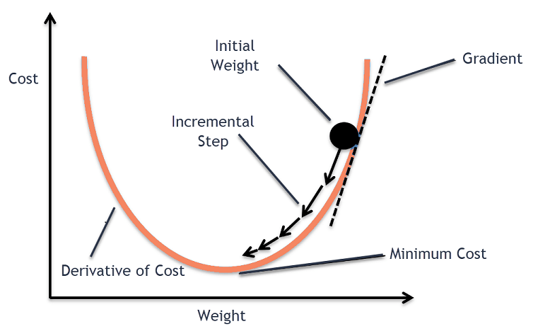
1. Initialization: We start at a random point in the parameter space.
2. Derivative Computation: The derivative (or gradient) gives the direction of steepest ascent.
3. Parameter Update: By moving in the opposite direction of the gradient and scaling the movement by the learning rate, we reduce the loss.
4. Convergence: The process is repeated until it converges to the minimum.

Importance of Convergence

It is essential to recognize when \ how sufficient conditions of convergence are met.

• Global vs. Local Minima: Gradient descent might converge to a local rather than the global minimum. This problem is more pronounced in non-convex loss functions.

• Convergence Rate: This is about how quick or slow the algorithm reaches equilibrium and will depend on the choice of learning rate, data, and model characteristics.

Fortunately, there exist strategies and techniques to enhance the algorithm to circumvent such obstacles. And, a successful convergence promises a solution that at least represents a local minimum of the loss function.

7. Describe the concept of the cost function and its role in gradient descent.

In Gradient Descent optimization, the primary task involves minimizing a Cost Function. This function maps the relationship between model parameters and the accuracy or error of predictions.

Role in Optimization

1. Discovering Optimal Parameters: The purpose of Gradient Descent is to identify model parameters that minimize the cost function, thereby making predictions as accurate as possible.

2. Quantifying Model Performance: The cost function acts as a measurable representation of the model's predictive accuracy or inaccuracy.

3. Continuous Improvement: Through iterations, gradient descent refines the model by systematically adjusting the parameters to minimize cost.

Common Cost Functions

Some datasets and machine learning tasks come with natural choices for the cost function. A few common ones include:

• Mean Squared Error (MSE): Ideal for regression tasks.
• Cross-Entropy (Log Loss): Suited for binary and multi-class classification tasks.
• Hinge Loss: Beneficial for binary classification, especially in Support Vector Machines.

Cost Function Overview

The cost function, represented as $J(\theta)$, measures the difference between predicted and actual values. The specific design of the cost function is determined by the nature of the ML task.

For instance, in a linear regression, the cost function $J(\theta)$ takes the form:

$$ J(\theta) = \frac{1}{2m} \sum_{i=1}^{m} \big( h_{\theta}(x^{(i)}) - y^{(i)} \big)^2 $$

where:

• $m$ is the number of training examples.
• $h_{\theta}(x^{(i)})$ is the predicted value.
• $y^{(i)}$ is the actual value.

Cost Function and Predictions

The key to minimizing the cost function is to refine the model's predictions. This is accomplished through a feedback mechanism, where the errors in predictions are used to update model parameters. The ultimate goal is to minimize the empirical risk, or the average error over the training data.

Minimizing the cost function is equivalent to finding the parameter set, denoted as $\theta^$ or $\beta^$, where the predictions align most closely with the actual values, thus optimizing the inductive bias of the model.

Process Illustration

1. Calculate Predictions: For each data point, use the current model parameters to make predictions.
2. Compute Errors: Find the discrepancies between predicted and actual values.
3. Evaluate Cost: Use the cost function to measure the overall error, which needs to be minimized.
4. Update Parameters: Using the gradient of the cost function, adjust model parameters to reduce errors in predictions.
5. Repeat: Steps 1-4 iteratively over the training data until the cost function is minimized.

Code Example: Mean Squared Error

Here is the Python code:

def mean_squared_error(predictions, actual):
    return np.mean((predictions - actual) ** 2)

# Calculate the cost using current parameter values and evaluate the performance
cost = mean_squared_error(model.predict(X_train), y_train)

# Adjust model parameters using gradient and update through backpropagation

8. Explain what a derivative tells us about the cost function in the context of gradient descent.

When we use derivative information in gradient descent, it enables us to find the direction of steepest descent in the multidimensional space. This guides the iterative process of cost function minimization, a fundamental step in optimizing machine learning models.

Importance of Accelerating Descent

• Time Efficiency: Instead of a full-scale search of the entire parameter space, the derivative helps identify the direction of fastest decrease in the cost function.

• Convergence: By focusing on the most promising regions, the algorithm is more likely to converge to the optimal solution. The derivative provides essential information for determining when to stop iteration, based on specific convergence criteria.

Key Roles of Derivatives in Gradient Descent

1. Global Orientation: The sign of the derivative indicates whether the function is increasing or decreasing. This drives the algorithm toward regions of lower cost.

2. Local Scale: The magnitude of the derivative (slope) provides immediate feedback on how steeply the cost function is changing. Large derivatives indicate steep inclines or declines, while small derivatives correspond to gentle slopes.

3. Rate of Change: Mathematically, the derivative (or gradient, in multi-dimensional spaces) specifies the rate of change of the cost function with respect to each model parameter. This rigorously defines the direction of steepest descent, as well as the step size based on the learning rate.

Code Example: Gradient Descent

Here is the Python code:

import numpy as np

# Define the cost function
def cost_function(x):
    return x**2 + 5  # Example function: f(x) = x^2 + 5

# Define the derivative of the cost function
def derivative(x):
    return 2*x  # Derivative of the above function: f'(x) = 2x

def gradient_descent(learning_rate, iterations):
    x = 0  # Initial guess for the minimum
    for _ in range(iterations):
        slope = derivative(x)
        step = learning_rate * slope
        x = x - step
    return x

learning_rate = 0.1
iterations = 100
optimal_x = gradient_descent(learning_rate, iterations)
print(optimal_x)

In this code, the derivative function computes the derivative of the cost function, and the gradient_descent function updates the parameter x iteratively, following the direction indicated by the derivative.

9. What is batch gradient descent, and when would you use it?

Batch Gradient Descent is a foundational optimization algorithm used in training supervised learning models. It computes the gradients of the cost function for the entire dataset in each iteration.

Core Idea

The algorithm involves three fundamental computations:

1. Cost Function: Measures how well the model predicts the training data.

2. Model Predictions: The algorithm uses the model's input to make predictions.

3. Gradient Computation: This is the most computation-intensive step. The algorithm computes the gradient of the cost function with respect to the model's parameters.

Advantages and Disadvantages

• Advantages:

  • Mathematically Guaranteed to Converge: Under certain conditions, Batch GD will converge to the global minimum.
  • Pareto Efficiency: Maintains a record of the best update so far.
  • Accurate: Computes precise gradients with the entire dataset.

• Disadvantages:

  • Computationally Inefficient: Processing the entire dataset can be slow and memory-intensive, especially with large datasets.
  • Lack of Stochasticity: May get stuck in sharp or narrow minima and doesn't benefit directly from the regularization effect of noise in 'stochastic' methods.
  • Memory Requirements: It requires data to fit in memory.

Code Example: Batch Gradient Descent

Here is the Python code:

def compute_gradient(parameters, data):
    # Your method for computing gradients goes here
    pass

def batch_gradient_descent(data, initial_parameters, learning_rate, num_iterations):
    parameters = initial_parameters
    for _ in range(num_iterations):
        gradients = compute_gradient(parameters, data)
        parameters -= learning_rate * gradients
    return parameters

10. Discuss the concept of stochastic gradient descent (SGD) and its advantages and disadvantages.

Stochastic Gradient Descent (SGD) is a variant of the traditional Gradient Descent algorithm designed to handle large datasets more efficiently.

How SGD Works

While traditional Gradient Descent calculates the gradient on the whole dataset to update parameters, SGD does it for individual or small sets of samples. This results in faster, but potentially noisier, convergence.

The algorithm entails these key steps:

1. Initialization: Set an initial parameter guess theta and configure learning rate alpha.

2. Random Selection: Choose a mini-batch or a single data point randomly.

3. Calculate Gradient: Compute the cost and partial derivatives with respect to each parameter for the chosen data points.

4. Update Parameters: Adjust each parameter based on the calculated gradient and the learning rate.

5. Convergence Checking: Repeat steps 2–4 until a stopping criterion is met.

Code Example: Stochastic Gradient Descent for Linear Regression

Here is the Python code:

import numpy as np

# Data preparation
X = 2 * np.random.rand(100, 1)
y = 4 + 3 * X + np.random.randn(100, 1)

X_b = np.c_[np.ones((100, 1)), X]

# SGD parameters
n_epochs = 50
t0, t1 = 5, 50  # hyperparameters

def learning_schedule(t):
    return t0 / (t + t1)

# SGD
theta = np.random.randn(2, 1)

for epoch in range(n_epochs):
    for i in range(100):
        random_index = np.random.randint(100)
        xi, yi = X_b[random_index:random_index+1], y[random_index:random_index+1]
        gradients = 2 * xi.T.dot(xi.dot(theta) - yi)
        eta = learning_schedule(epoch * 100 + i)
        theta = theta - eta * gradients

In this example, we use Stochastic Gradient Descent to find the parameters for a simple linear regression model.

Advantages of SGD

• Computation Efficiency: SGD processes smaller, randomly sampled data points, ideal for vast datasets.

• Memory Efficiency: With its mini-batch approach, SGD requires less memory, making it suitable for systems with memory constraints.

• Potential for Improved Generalization: The noise in parameter updates can make the model explore different local minima, leading to potentially better generalization.

Disadvantages of SGD

• Convergence to Local Minima: The noisiness can cause the algorithm to oscillate around the minimum, making it prone to getting stuck in local optima.

• Parameter Tuning Sensitivity: Choosing the ideal learning rate can be more challenging due to the noise, and it might require additional tuning of $t_0$ and $t_1$ in the learning schedule.

• May Converge to a Noisier Region: Due to its random nature, SGD might not reach the exact minimum achievable by traditional Gradient Descent methods.

11. What is mini-batch gradient descent, and how does it differ from other variants?

Mini-batch Gradient Descent (Batch GD) is a compromise between Stochastic GD and Batch GD methods, aiming to reconcile their individual strengths.

Key Characteristics

Batch GD

• Update Frequency: After processing the entire dataset
• Robustness: Provides accurate updates leveraging complete dataset information but might converge slowly, particularly for extensive datasets.

Stochastic GD

• Update Frequency: After processing each data point
• Robustness: Efficient for large datasets but can be erratic and struggle near convergence, as each data point's influence can be too significant.

Mini-batch GD

• Update Frequency: After processing a subset (mini-batch) of the dataset
• Robustness: Balanced approach that offers speed and stability.

Algorithm for Mini-Batch Gradient Descent

1. Initialize: Choose learning rate $\alpha$ and define mini-batch size.
2. Randomize Data: Shuffle the dataset to form mini-batches.
3. Iterate: For each mini-batch, update parameters.
4. Convergence Check: Discontinue once stopping criteria are met.

Code Example: Mini-Batch Gradient Descent

Here is the Python code:

import numpy as np

def mini_batch_gradient_descent(X, y, theta, learning_rate=0.01, iterations=100, batch_size=10):
    m = len(y)  # Number of training examples
    num_batches = int(m / batch_size)
    for _ in range(iterations):
        # Shuffle data and split into mini-batches
        permutation = np.random.permutation(m)
        X_shuffled = X[permutation]
        y_shuffled = y[permutation]
        for i in range(num_batches):
            start = i * batch_size
            end = min(start + batch_size, m)
            X_batch, y_batch = X_shuffled[start:end], y_shuffled[start:end]
            # Compute gradient and update parameters
            gradient = 1 / batch_size * X_batch.T.dot(X_batch.dot(theta) - y_batch)
            theta -= learning_rate * gradient
    return theta

12. Explain how momentum can help in accelerating gradient descent.

Gradient Descent (GD) in its basic form updates model parameters $\theta$ in small steps using the present gradient of the cost function. While this method is reliable, it can sometimes be slow to converge, especially in the presence of noise or if the cost function has a complex, elongated shape.

The Need for Acceleration

In these scenarios, the step size, or learning rate, often needs to be kept small to prevent overshooting past the minimum. However, a small learning rate leads to slow convergence.

Researchers have developed momentum as an enhancement to traditional GD, aiming to address these issues.

Core Concept: Momentum

In momentum-aided GD, the next update to the parameters, $\theta$, gets a "boost" from the previous parameter update as well. Mathematically, the parameter update rule becomes:

$$ \Delta \theta = \mu \cdot \Delta \theta_{\text{previous}} - \text{learning rate} \cdot \nabla_\theta J( \theta ) $$

$$ \theta \leftarrow \theta + \Delta \theta $$

where $\mu$ is the momentum term, usually a value between 0 and 1.

1. The first term, $\mu \cdot \Delta \theta_{\text{previous}}$, represents the "momentum" or accumulated velocity from previous updates. If the path to the minimum is long and winding, this momentum ensures a more consistent direction of movement, helping it navigate through plateaus and local minima more effectively.

2. The second term, $- \text{learning rate} \cdot \nabla_\theta J( \theta )$, is the traditional gradient term, indicating the current direction in the parameter space that leads to a decrease in the cost function.

Choosing the Right Momentum Value

Typically, a momentum value, $\mu$, between 0.8 and 0.99 is effective across various scenarios. This range ensures that the algorithm has more stable and consistent movement with less sensitivity to individual gradient estimates.

13. Describe the difference between Adagrad, RMSprop, and Adam optimizers.

Adagrad, RMSprop, and Adam optimizers are all variations of the stochastic gradient descent (SGD) algorithm that aim to improve its efficiency and convergence characteristics.

Each optimizer has its unique features, benefits, and drawbacks, catering to different datasets and models. Let's take a closer look at each.

Adagrad

• Adagrad adapts the learning rate for each parameter $w_i$ based on the accumulated squared gradient for that parameter up to the current time step $t$:

$$ G_{t,ii} \leftarrow G_{t-1,ii} + \nabla w_i \cdot \nabla w_i $$ $$ w_{t+1,i} \leftarrow w_{t,i} - \frac{\eta}{\sqrt{G_{t,ii} + \epsilon}} \cdot \nabla w_i $$

• The strengths of individual parameters are naturally taken into account. However, this approach can lead to an excessively small learning rate over time.

RMSprop

• RMSprop addresses Adagrad's issue of the monotonically decreasing learning rate by accumulating only a fraction $\rho$ of previous squared gradients and updating the parameters based directly:

$$ G_{t,ii} \leftarrow \rho \cdot G_{t-1,ii} + (1 - \rho) \cdot \nabla w_i \cdot \nabla w_i $$ $$ w_{t+1,i} \leftarrow w_{t,i} - \frac{\eta}{\sqrt{G_{t,ii} + \epsilon}} \cdot \nabla w_i $$

• This method ensures a balance between adapting to recent gradients and maintaining a sufficient learning rate.

Adam

• Adam further improves upon RMSprop by incorporating adaptive momentum. It computes the gradients' first and second moments, giving rise to the $m_t$ and $v_t$ variables.

• The unbiased estimation of $m_t$ and $v_t$ at the start of the optimization addresses Adam's bias towards zero, especially during early iterations:

$ m_t \leftarrow \beta_1 \cdot m_{t-1} + (1 - \beta_1) \cdot \nabla w_t $ $ v_t \leftarrow \beta_2 \cdot v_{t-1} + (1 - \beta_2) \cdot \nabla w_t \cdot \nabla w_t $ $ \hat{m}_t = \frac{m_t}{1 - \beta_1^t} $ $ \hat{v}t = \frac{v_t}{1 - \beta_2^t} $ $ w{t+1} = w_t - \frac{\eta}{\sqrt{\hat{v}_t} + \epsilon} \cdot \hat{m}_t $

• Adam has become a popular choice in recent years due to its robust performance across a wide range of ML tasks.

14. What is the problem of vanishing gradients, and how does it affect gradient descent?

Let's look at how vanishing gradients can impede the performance of gradient-based optimization algorithms and at the solutions designed to mitigate this issue.

The Issue: Vanishing Gradients

In deep neural networks, particularly those with many layers, multiplicative changes through layers can cause coding numerical reasoning difficulties. This results from gradients that become extremely small as they propagate backward through the network.

The problem is especially acute in activation functions like sigmoid or tanh, which saturate to very flat regions for large positive or negative inputs. Small gradients provide less information to update the model's earlier layers, leading to slower learning and, at times, little learning at all.

Impact on Models

• Poor Initialization: Vanishing gradients can lead to sub-optimal performance during model training if initial weights set the network in regions where gradients are minimal.

• Long Valleys: The emergent valleys or troughs in the loss landscape become flatter as the network depth increases, compelling gradient-based methods to become stuck in these regions.

• Saturated Outputs: Hidden layers in a network characterized by non-representative, excessively large, or tiny activations due to momentum transfer might cease learning.

Solutions

Several techniques aim to address vanishing gradients:

• Activation Function Selection: Using activation functions less prone to saturation such as ReLU or their variants.

• Proper Weight Initialization: Methods like the Xavier/Glorot initializer help to initialize the weights such that the variance in activations across layers remains consistent.

• Batch Normalization: This method introduces parameters that scale and translate the network's outputs at various layers and mitigate internal covariate shift.

• Gated Recurrent Units (GRUs) and Long Short-Term Memory (LSTM) networks: Specialized models formulated to alleviate issues related to vanishing gradients in recurrent neural networks.

• Weight Regularization: Techniques like L1 or L2 regularization restrict the model's parameter space, potentially avoiding large swings that yield vanishing gradients.

• Residual Connections: These connections bypass one or more layers, representing an unobstructed path, which can help alleviate vanishing gradients.

• Vanishing and Exploding Gradient: There are primarily two issues(Vanishing Gradient and Exploding Gradient) that a come as a problematic side-effect especially while working with deeper neural network. Use of modern activation functions and a tactic called clippping which restricts the gradient value with a specified range, are some of the solution to deal with underperforming deep neural networks.

• Clipping: Mechanisms such as gradient clipping impose boundaries on the magnitude of the gradients, constraining the likelihood of extremely tiny gradients to some extent.UTF-8

15. How can gradient clipping help in training deep learning models?

Gradient clipping combats issues related to vanishing or exploding gradients during deep learning model training.

Causes and Consequences of Unstable Gradients

• Vanishing Gradients: Occur in deep networks when early layers receive tiny gradients during backpropagation. This often results in slow convergence or even stagnation.

• Exploding Gradients: Conversely, this involves exceptionally large gradients, possibly leading to numerical instability during optimization.

Mechanism of Gradient Clipping

When the L2 norm of the gradient vector surpasses a defined threshold, the vector gets rescaled to ensure it remains within the set range. Doing so maintains the stability of the training process.

Step-by-Step Gradient Clipping Process

1. Gradient Computation: Derive model parameter gradients using backpropagation.
2. Calculate Norm: Measure the L2 norm (magnitude) of the gradient vector.
3. Threshold Comparison: If the computed norm exceeds the preset threshold, scale the gradient vector to ensure it remains within the limit.
4. Optimization Step: Update model parameters using the clipped gradient.

Code Example: Gradient Clipping

Here is the Python code:

# Define the model
model = SomeDeepLearningModel()

# Set learning rate and optimizer
learning_rate = 0.01
optimizer = tf.keras.optimizers.SGD(learning_rate)

# Define threshold for gradient clipping
clip_norm = 1.0

# Training loop
for epoch in range(num_epochs):
    for batch in train_dataset:
        with tf.GradientTape() as tape:
            # Forward pass
            output = model(batch)
            # Compute loss
            loss = compute_loss(output, batch)
        # Get gradients
        gradients = tape.gradient(loss, model.trainable_variables)
        # Apply gradient clipping
        clipped_gradients, _ = tf.clip_by_global_norm(gradients, clip_norm) 
        # Update model parameters
        optimizer.apply_gradients(zip(clipped_gradients, model.trainable_variables))

Explore all 50 answers here 👉 Devinterview.io - Gradient Descent